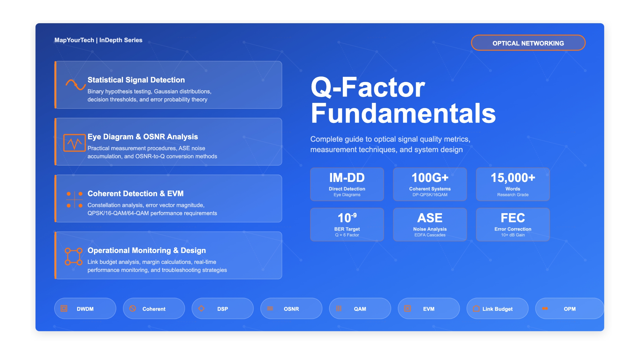
Q-Factor Fundamentals: Complete Guide to Optical Signal Quality Metrics

A comprehensive research-grade exploration of quality factor theory, measurement, and application in modern coherent optical communication systems

In modern coherent optical systems operating at 100 Gb/s, 400 Gb/s, and beyond, the Q-factor serves multiple roles. It functions as a design metric during system planning, helping engineers determine required optical signal-to-noise ratios (OSNR) for target bit error rates (BER). During deployment, Q-factor measurements validate that installed systems meet performance specifications. In operational networks, real-time Q-factor monitoring enables proactive identification of degrading links before service-affecting failures occur. Understanding Q-factor fundamentals is therefore essential for anyone working with optical transmission systems.

The relationship between Q-factor and bit error rate is rooted in statistical decision theory. When a receiver attempts to distinguish between transmitted binary ones and zeros, noise and other impairments cause the received signal levels to fluctuate. The Q-factor quantifies how well separated these signal distributions are relative to their spread (standard deviation). A higher Q-factor indicates better separation and lower error probability. This seemingly simple metric encapsulates the complex interplay of transmitter quality, fiber impairments, amplifier noise, receiver sensitivity, and modulation format characteristics.

Historically, Q-factor emerged from intensity-modulated direct-detection (IM-DD) systems where it could be measured directly from eye diagrams by comparing signal levels and noise statistics. With the transition to coherent detection and advanced modulation formats such as QPSK, 16-QAM, and 64-QAM, the definition and measurement of Q-factor have evolved significantly. Modern digital signal processing (DSP) techniques enable Q-factor estimation from constellation diagrams and error vector magnitude (EVM) measurements, providing insights that extend beyond simple intensity detection.

1.1 Scope and Objectives

This comprehensive guide examines Q-factor from multiple perspectives, providing both theoretical foundations and practical applications. The scope includes the mathematical basis of Q-factor in signal detection theory, its relationship to OSNR and BER, measurement techniques for different modulation formats, and the role of Q-factor in system design and performance monitoring. The guide addresses both traditional IM-DD systems and modern coherent systems, recognizing that different approaches are required for different technology generations.

The primary objectives are to provide network engineers with a deep understanding of what Q-factor represents physically, how it relates to other performance metrics, and how to use it effectively for system design and troubleshooting. For research professionals, the guide explores the theoretical foundations, including the statistical assumptions underlying Q-factor calculations and their limitations. For operations teams, practical guidance on Q-factor monitoring, threshold setting, and interpretation in production networks is provided.

1.2 Significance in Modern Optical Networks

Modern optical networks face unprecedented challenges in maintaining signal quality. Long-haul submarine cables span thousands of kilometers with dozens of optical amplifiers, each adding noise. Metro networks accommodate dynamic traffic patterns with frequent wavelength additions and deletions. Data center interconnects demand maximum capacity over relatively short distances but with minimal latency and power consumption. In each scenario, Q-factor provides essential visibility into signal quality and system margins.

The shift toward software-defined networking (SDN) and network automation amplifies the importance of accurate Q-factor measurement. Automated path computation engines need reliable quality metrics to make routing decisions. Margin-adaptive systems adjust modulation formats based on measured Q-factor to optimize capacity. Predictive maintenance systems analyze Q-factor trends to schedule preventive interventions before failures occur. These applications all depend on understanding what Q-factor represents and how to measure it accurately.

The evolution of modulation formats introduces additional complexity. Different formats (BPSK, QPSK, 16-QAM, 64-QAM) have different OSNR requirements for the same target BER, and these relationships must be understood to properly interpret Q-factor measurements. Polarization-division multiplexing (PDM) doubles spectral efficiency but introduces polarization-dependent impairments that affect Q-factor. Probabilistic constellation shaping optimizes information rates but changes the statistical properties that Q-factor measurements assume. Modern optical engineers must navigate these complexities with a solid foundation in Q-factor fundamentals.

The concept of quality factor in optical communications traces its roots to early work in electrical signal detection and information theory. Claude Shannon's groundbreaking 1948 paper establishing the mathematical theory of communication provided the theoretical foundation for understanding the relationship between signal-to-noise ratio and channel capacity. However, the specific application of Q-factor to optical systems emerged later, driven by the unique characteristics of optical transmission and detection.

2.1 Early Optical Systems and Eye Diagrams

In the 1980s and 1990s, optical communication systems primarily used on-off keying (OOK) with direct detection. Engineers characterized these systems using oscilloscopes displaying eye diagrams, which provided visual representations of signal quality. The eye opening, measured as the vertical distance between the mean one level and mean zero level relative to the noise margins, became a natural quality metric. This visual representation led to the formalization of Q-factor as a quantitative measure.

The classical Q-factor definition for IM-DD systems emerged from analyzing these eye diagrams statistically. By measuring the mean signal levels for ones (S₁) and zeros (S₀) along with their respective standard deviations (σ₁ and σ₀), engineers could calculate a quality factor that predicted bit error probability. This approach proved particularly valuable because it could be performed with relatively simple test equipment and provided direct insight into the physical factors limiting system performance.

Early systems operated at relatively modest data rates (155 Mb/s, 622 Mb/s, 2.5 Gb/s) over limited distances, making Q-factor measurements straightforward. The dominant noise source was typically thermal noise in the receiver, and chromatic dispersion could often be neglected or compensated with simple dispersion-compensating fiber. As systems evolved to 10 Gb/s and beyond, additional impairments became significant, and the relationship between Q-factor and actual system performance became more complex.

2.2 Transition to DWDM and Amplified Systems

The introduction of dense wavelength division multiplexing (DWDM) and erbium-doped fiber amplifiers (EDFAs) in the mid-1990s fundamentally changed optical system design. Multiple wavelength channels sharing the same fiber introduced crosstalk and nonlinear impairments. Optical amplification enabled unprecedented transmission distances but added amplified spontaneous emission (ASE) noise that became the dominant impairment. These changes required new approaches to Q-factor analysis.

In amplified DWDM systems, optical signal-to-noise ratio (OSNR) emerged as a critical parameter directly related to ASE noise accumulation. The relationship between OSNR and Q-factor became a central concern for system designers. Understanding that Q-factor degraded with accumulated ASE noise allowed engineers to predict system performance based on amplifier noise figures, span losses, and total transmission distance. This predictive capability proved essential for designing long-haul systems with acceptable performance.

The relationship between OSNR and Q-factor depends on several factors including extinction ratio, optical and electrical filtering, and the statistical properties of the noise. For ideal systems with perfect extinction ratio and matched filtering, simple formulas relate OSNR to Q-factor. However, real systems deviate from these ideal conditions, requiring more sophisticated analysis. The development of numerical simulation tools enabled more accurate predictions, but Q-factor remained the fundamental metric linking OSNR to BER.

2.3 Coherent Detection and Digital Signal Processing

The emergence of coherent detection with digital signal processing (DSP) around 2008 represented another paradigm shift. Coherent receivers provide access to both amplitude and phase information, enabling sophisticated modulation formats (QPSK, 16-QAM, 64-QAM) that increase spectral efficiency. DSP compensates for chromatic dispersion, polarization mode dispersion, and other linear impairments electronically, eliminating the need for optical compensation. These advances required new approaches to Q-factor measurement and interpretation.

In coherent systems, the traditional eye diagram becomes less meaningful for multilevel modulation formats. Instead, constellation diagrams showing the distribution of received symbols in the complex plane provide analogous visual information. The concept of error vector magnitude (EVM), borrowed from wireless communications, quantifies the deviation of received symbols from their ideal locations. Q-factor can be estimated from EVM measurements, but the relationship depends on the modulation format and the nature of the impairments.

Modern DSP-based receivers can estimate Q-factor from the fully equalized signal, after compensation for chromatic dispersion, PMD, and frequency/phase offsets. This "post-DSP Q-factor" represents the quality of the signal at the decision point, providing the most direct prediction of BER. However, monitoring systems may also measure "pre-DSP Q-factor" or "optical Q-factor" to assess the quality of the optical signal before electronic compensation. Understanding the distinctions between these different Q-factor definitions is essential for proper interpretation.

3.1 Statistical Signal Detection Theory

The theoretical foundation of Q-factor lies in binary hypothesis testing from statistical decision theory. When a receiver attempts to decode a binary signal, it must decide whether a transmitted bit was a one or a zero based on the received signal level, which is corrupted by noise and other impairments. The optimal decision threshold minimizes the probability of error, and the Q-factor quantifies how well the signal distributions are separated relative to their overlap.

Consider a binary communication system where the transmitter sends either a signal representing a logical one (with mean power S₁) or a signal representing a logical zero (with mean power S₀). Noise and other random impairments cause the received signal to fluctuate around these mean values. If we model the noise as additive Gaussian noise, the received signal for a transmitted one follows a Gaussian distribution with mean S₁ and standard deviation σ₁. Similarly, received zeros follow a Gaussian distribution with mean S₀ and standard deviation σ₀.

The receiver must establish a decision threshold I_d such that received signals above the threshold are decoded as ones and signals below the threshold are decoded as zeros. Errors occur when noise causes a transmitted one to fall below the threshold (causing a one-to-zero error) or when noise causes a transmitted zero to exceed the threshold (causing a zero-to-one error). The total bit error rate is the sum of these two error probabilities, weighted by the probability of transmitting ones and zeros.

Q-Factor Definition for Binary Signaling:

Q = (S1 - S0) / (σ1 + σ0)

Where:
S1 = Mean signal level for transmitted ones
S0 = Mean signal level for transmitted zeros  
σ1 = Standard deviation of noise for ones
σ0 = Standard deviation of noise for zeros

This formula represents the signal separation relative to the total noise spread.

The Q-factor represents the distance between the two signal means in units of the combined noise standard deviation. A higher Q-factor indicates better separation between the signal distributions, resulting in lower error probability. For equally likely ones and zeros with equal noise variances (σ₁ = σ₀ = σ), the formula simplifies to Q = (S₁ - S₀) / (2σ), showing that Q is proportional to the signal-to-noise ratio.

3.2 Relationship Between Q-Factor and Bit Error Rate

The relationship between Q-factor and bit error rate derives from the properties of Gaussian probability distributions. Assuming Gaussian noise statistics and an optimally placed decision threshold, the bit error rate can be expressed in terms of the complementary error function (erfc) of the Q-factor. This mathematical relationship provides the critical link between the physical measurement of signal quality and the practical metric of system performance.

BER-to-Q-Factor Relationship:

BER = (1/2) × erfc(Q / √2)

For Q ≥ 3, this can be approximated as:

BER ≈ exp(-Q2/2) / (Q × √(2π))

Common BER-Q-factor pairs:
Q = 6.0  → BER ≈ 10-9
Q = 7.0  → BER ≈ 10-12  
Q = 8.0  → BER ≈ 10-15

In dB scale: QdB = 20 × log10(Q)
QdB = 15.6 dB corresponds to Q = 6.0 (BER = 10-9)

This exponential relationship between Q and BER means that small changes in Q-factor translate to large changes in bit error rate. An improvement of 1 dB in Q-factor (from 15.6 dB to 16.6 dB, corresponding to Q from 6.0 to 6.8) reduces BER by more than an order of magnitude (from 10^-9 to approximately 10^-11). This sensitivity makes Q-factor a powerful tool for system optimization but also demands accurate measurement techniques.

The relationship assumes several ideal conditions: Gaussian noise statistics, optimal threshold placement, and independent errors. Real optical systems may deviate from these assumptions. Non-Gaussian noise (from crosstalk or nonlinear effects), suboptimal threshold setting, or error correlation can cause the actual BER to differ from the predicted value. Forward error correction (FEC) adds redundancy that reduces post-FEC BER below the raw BER predicted by Q-factor, typically by several orders of magnitude.

3.3 Q-Factor in Different Modulation Formats

While Q-factor originated in binary intensity modulation systems, the concept extends to multilevel modulation formats used in coherent systems. However, the relationship between Q-factor, OSNR, and BER depends on the specific modulation format. BPSK (binary phase shift keying), QPSK (quadrature phase shift keying), 16-QAM (quadrature amplitude modulation), and higher-order formats each have different geometries in signal space, affecting their noise tolerance.

For BPSK and QPSK modulation, symbols are positioned at equal distances from the origin in the constellation diagram. The minimum Euclidean distance between symbols determines the noise tolerance. In QPSK, each symbol carries two bits, but because symbols are separated by the same minimum distance as in BPSK operating at the same average power, the per-bit SNR requirement remains similar. This makes QPSK particularly attractive, doubling spectral efficiency with minimal penalty.

Sanjay Yadav

Optical Communications & Network Automation Expert | Author of 3 Books for Optical Engineers | Founder, MapYourTech

Optical networking engineer with nearly two decades of experience across DWDM, OTN, coherent optics, submarine systems, and cloud infrastructure. Founder of MapYourTech. Read full bio →

Follow on LinkedIn

Related Articles on MapYourTech

Free · Jul 11, 2026

Connector Types and Their Loss Budgets: SC, LC, MPO

Automation · Jul 11, 2026

Cooled vs Uncooled Lasers: The Pluggable Power Trade-off

Automation · Jul 11, 2026

Automation Blast Radius: Scoping What a Bad Intent Can Touch

Analysis · Jul 11, 2026

ASE Channel Loading: Running a Line System Full From Day One