 MapYourTech | InDepth Series
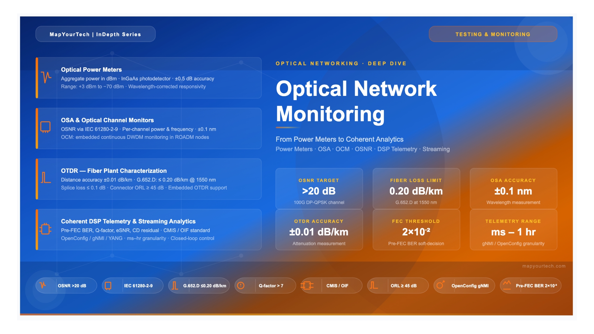
Optical Network Monitoring: From Power Meters to Coherent Analytics
A practical overview of optical monitoring tools — power meters, Optical Spectrum Analyzers, optical channel monitors, inline Optical Signal-to-Noise Ratio monitors, and modern coherent Digital Signal Processor-based performance telemetry.
Introduction
An optical network operates on physical signals — photons propagating through glass. Unlike packet networks where a routing table entry can be inspected in software, the health of an optical link depends on power levels, noise floors, wavelength accuracy, and a range of physical impairments that can only be observed in the optical domain itself. When a wavelength degrades silently over weeks, or a connector fault appears at kilometre 80 of a span, the tools that expose these conditions determine whether the operator finds out proactively or after service has already dropped.
Optical performance monitoring encompasses a family of instruments and techniques that have evolved dramatically over three decades — from handheld optical power meters used during fiber splicing, to Optical Spectrum Analyzers (OSAs) characterizing multi-channel Dense Wavelength Division Multiplexing (DWDM) systems, to today's coherent Digital Signal Processors (DSPs) that continuously extract Optical Signal-to-Noise Ratio (OSNR), pre-Forward Error Correction (FEC) Bit Error Rate (BER), chromatic dispersion, and polarization state directly from live traffic, with results streamed to analytics platforms via open interfaces.
This article surveys the complete toolkit — instrument by instrument — covering operating principles, what each tool can and cannot measure, where it sits in the network, and how the monitoring landscape has shifted as coherent optics, pluggable modules, and software-defined control have converged. The target reader is an engineer who already understands fiber optics and DWDM fundamentals and wants a clear, technically grounded map of monitoring approaches across the full lifecycle of an optical network.
Why Optical Monitoring Exists
Optical signals change over time and distance. Fiber ages, connectors accumulate contamination, amplifier gain profiles shift, laser temperatures fluctuate, and traffic patterns alter the distribution of power across a DWDM comb. Without observation, none of these changes are visible until they cross a threshold that produces alarms or errors. By that point, the degradation has typically been accumulating for hours, days, or weeks.
The parameters that drift in a live optical network fall into several categories. Optical power decreases due to fiber aging, connector contamination, or component wear. Wavelength shifts when laser temperature control loses accuracy or filter passbands drift with thermal cycling. OSNR degrades as amplifier noise accumulates along a route, particularly when span loss increases because of fiber deterioration, forcing amplifiers to operate at higher gain and therefore higher noise figure. Chromatic dispersion (CD) accumulates deterministically with distance but becomes relevant again when a route changes through Reconfigurable Optical Add-Drop Multiplexer (ROADM) reconfiguration. Polarization Mode Dispersion (PMD) is a stochastic impairment influenced by fiber geometry, mechanical stress, and temperature.
Network failures fall broadly into two types. Catastrophic failures — fiber cuts, amplifier failure, laser death — manifest without warning and immediately remove traffic. Degradation failures develop slowly: a gradual OSNR decline, creeping FEC symbol error count, or slowly rising BER that may not trigger alarms for weeks while consuming margin. A well-designed monitoring architecture addresses both: event-triggered alarms for catastrophic events and continuous trending for degradation detection.
Monitoring vs. Testing — A Key Distinction
Test instruments (portable OSAs, OTDRs, BER testers) are used during commissioning and troubleshooting. They are brought to the network as needed and do not operate continuously. Monitoring instruments (embedded OCMs, DSP telemetry, in-line optical performance monitors) operate continuously as part of the deployed network. Both categories are covered in this article because an engineer needs to understand both when characterizing a link and when operating it in service.
The consequences of inadequate monitoring are concrete. Insufficient visibility means that operators cannot detect sudden faults early, cannot perform root cause analysis on gradual degradations, and must engineer excessively conservative system margins — effectively over-building the network to tolerate problems that a well-monitored system could correct dynamically. As networks scale to 400G, 800G, and beyond — with higher-order modulation formats that consume OSNR margin rapidly — the ability to observe and react to physical layer health becomes more important, not less.
Optical Power Meters — The Foundation
The optical power meter is the simplest and most fundamental optical measurement instrument. It converts incident optical power into an electrical current via a photodetector — typically an InGaAs photodiode for telecom wavelengths — and reports the result in dBm or milliwatts. Nothing about the signal's wavelength, modulation format, or OSNR is observable with a power meter alone; it integrates all incident light across its active area and its wavelength response range.
3.1 Operating Principle and Measurement Range
A photodiode generates a photocurrent proportional to incident optical power. The detector's responsivity — expressed in amperes per watt — determines how much current is produced per unit of optical power, and it is wavelength-dependent. For single-mode telecom applications in the C-band (1530–1565 nm) and L-band (1565–1625 nm), InGaAs detectors provide responsivities in the range of approximately 0.85–0.95 A/W, though the exact value depends on device design. The resulting current is amplified and converted to a power reading, typically displayed in dBm referenced to 1 milliwatt.
Read the Full Analysis with Premium
The remaining 89% of this article — the design numbers, trade-offs and field guidance — is part of MapYourTech Premium, along with the full premium library, courses and professional tools.