Tag

Network Design

Browsing

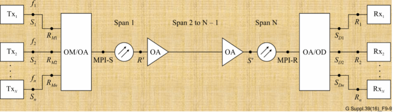
Optical networks are the backbone of the internet, carrying vast amounts of data over great distances at the speed of light. However, maintaining signal quality over long fiber runs is a challenge due to a phenomenon known as noise concatenation. Let’s delve into how amplified spontaneous emission (ASE) noise affects Optical Signal-to-Noise Ratio (OSNR) and the performance of optical amplifier chains.

The Challenge of ASE Noise

ASE noise is an inherent byproduct of optical amplification, generated by the spontaneous emission of photons within an optical amplifier. As an optical signal traverses through a chain of amplifiers, ASE noise accumulates, degrading the OSNR with each subsequent amplifier in the chain. This degradation is a crucial consideration in designing long-haul optical transmission systems.

Understanding OSNR

OSNR measures the ratio of signal power to ASE noise power and is a critical parameter for assessing the performance of optical amplifiers. A high OSNR indicates a clean signal with low noise levels, which is vital for ensuring data integrity.

Reference System for OSNR Estimation

As depicted in Figure below), a typical multichannel N span system includes a booster amplifier, N−1 line amplifiers, and a preamplifier. To simplify the estimation of OSNR at the receiver’s input, we make a few assumptions:

Representation of optical line system interfaces (a multichannel N-span system)
  • All optical amplifiers, including the booster and preamplifier, have the same noise figure.
  • The losses of all spans are equal, and thus, the gain of the line amplifiers compensates exactly for the loss.
  • The output powers of the booster and line amplifiers are identical.

Estimating OSNR in a Cascaded System

E1: Master Equation For OSNR

E1: Master Equation For OSNR

Pout is the output power (per channel) of the booster and line amplifiers in dBm, L is the span loss in dB (which is assumed to be equal to the gain of the line amplifiers), GBA is the gain of the optical booster amplifier in dB, NFis the signal-spontaneous noise figure of the optical amplifier in dB, h is Planck’s constant (in mJ·s to be consistent with Pout in dBm), ν is the optical frequency in Hz, νr is the reference bandwidth in Hz (corresponding to c/Br ), N–1 is the total number of line amplifiers.

The OSNR at the receivers can be approximated by considering the output power of the amplifiers, the span loss, the gain of the optical booster amplifier, and the noise figure of the amplifiers. Using constants such as Planck’s constant and the optical frequency, we can derive an equation that sums the ASE noise contributions from all N+1 amplifiers in the chain.

Simplifying the Equation

Under certain conditions, the OSNR equation can be simplified. If the booster amplifier’s gain is similar to that of the line amplifiers, or if the span loss greatly exceeds the booster gain, the equation can be modified to reflect these scenarios. These simplifications help network designers estimate OSNR without complex calculations.

1)          If the gain of the booster amplifier is approximately the same as that of the line amplifiers, i.e., GBA » L, above Equation E1 can be simplified to:

osnr_2

E1-1

2)          The ASE noise from the booster amplifier can be ignored only if the span loss L (resp. the gain of the line amplifier) is much greater than the booster gain GBA. In this case Equation E1-1 can be simplified to:

E1-2

3)          Equation E1-1 is also valid in the case of a single span with only a booster amplifier, e.g., short‑haul multichannel IrDI in Figure 5-5 of [ITU-T G.959.1], in which case it can be modified to:

E1-3

4)          In case of a single span with only a preamplifier, Equation E1 can be modified to:

Practical Implications for Network Design

Understanding the accumulation of ASE noise and its impact on OSNR is crucial for designing reliable optical networks. It informs decisions on amplifier placement, the necessity of signal regeneration, and the overall system architecture. For instance, in a system where the span loss is significantly high, the impact of the booster amplifier on ASE noise may be negligible, allowing for a different design approach.

Conclusion

Noise concatenation is a critical factor in the design and operation of optical networks. By accurately estimating and managing OSNR, network operators can ensure signal quality, minimize error rates, and extend the reach of their optical networks.

In a landscape where data demands are ever-increasing, mastering the intricacies of noise concatenation and OSNR is essential for anyone involved in the design and deployment of optical communication systems.

References

https://www.itu.int/rec/T-REC-G/e

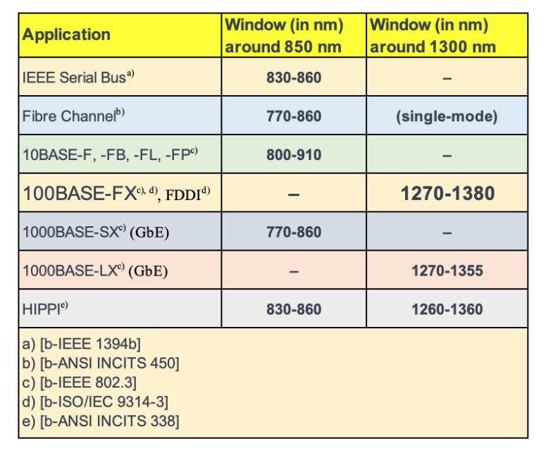
While single-mode fibers have been the mainstay for long-haul telecommunications, multimode fibers hold their own, especially in applications where short distance and high bandwidth are critical. Unlike their single-mode counterparts, multimode fibers are not restricted by cut-off wavelength considerations, offering unique advantages.

The Nature of Multimode Fibers

Multimode fibers, characterized by a larger core diameter compared to single-mode fibers, allow multiple light modes to propagate simultaneously. This results in modal dispersion, which can limit the distance over which the fiber can operate without significant signal degradation. However, multimode fibers exhibit greater tolerance to bending effects and typically showcase higher attenuation coefficients.

Wavelength Windows for Multimode Applications

Multimode fibers shine in certain “windows,” or wavelength ranges, which are optimized for specific applications and classifications. These windows are where the fiber performs best in terms of attenuation and bandwidth.

#multimodeband

IEEE Serial Bus (around 850 nm): Typically used in consumer electronics, the 830-860 nm window is optimal for IEEE 1394 (FireWire) connections, offering high-speed data transfer over relatively short distances.

Fiber Channel (around 770-860 nm): For high-speed data transfer networks, such as those used in storage area networks (SANs), the 770-860 nm window is often used, although it’s worth noting that some applications may use single-mode fibers.

Ethernet Variants:

  • 10BASE (800-910 nm): These standards define Ethernet implementations for local area networks, with 10BASE-F, -FB, -FL, and -FP operating within the 800-910 nm range.
  • 100BASE-FX (1270-1380 nm) and FDDI (Fiber Distributed Data Interface): Designed for local area networks, they utilize a wavelength window around 1300 nm, where multimode fibers offer reliable performance for data transmission.
  • 1000BASE-SX (770-860 nm) for Gigabit Ethernet (GbE): Optimized for high-speed Ethernet over multimode fiber, this application takes advantage of the lower window around 850 nm.
  • 1000BASE-LX (1270-1355 nm) for GbE: This standard extends the use of multimode fibers into the 1300 nm window for Gigabit Ethernet applications.

HIPPI (High-Performance Parallel Interface): This high-speed computer bus architecture utilizes both the 850 nm and the 1300 nm windows, spanning from 830-860 nm and 1260-1360 nm, respectively, to support fast data transfers over multimode fibers.

Future Classifications and Studies

The classification of multimode fibers is a subject of ongoing research. Proposals suggest the use of the region from 770 nm to 910 nm, which could open up new avenues for multimode fiber applications. As technology progresses, these classifications will continue to evolve, reflecting the dynamic nature of fiber optic communications.

Wrapping Up: The Place of Multimode Fibers in Networking

Multimode fibers are a vital part of the networking world, particularly in scenarios that require high data rates over shorter distances. Their resilience to bending and capacity for high bandwidth make them an attractive choice for a variety of applications, from high-speed data transfer in industrial settings to backbone cabling in data centers.

As we continue to study and refine the classifications of multimode fibers, their role in the future of networking is guaranteed to expand, bringing new possibilities to the realm of optical communications.

References

https://www.itu.int/rec/T-REC-G/e

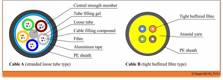
The world of optical communication is intricate, with different cable types designed for specific environments and applications. Today, we’re diving into the structure of two common types of optical fiber cables, as depicted in Figure below, and summarising the findings from an appendix that examined their performance.

cableA_B
#cable

Figure

Cable A: The Stranded Loose Tube Outdoor Cable

Cable A represents a quintessential outdoor cable, built to withstand the elements and the rigors of outdoor installation. The cross-section of this cable reveals a complex structure designed for durability and performance:

  • Central Strength Member: At its core, the cable has a central strength member that provides mechanical stability and ensures the cable can endure the tensions of installation.
  • Tube Filling Gel: Surrounding the central strength member are buffer tubes secured with a tube filling gel, which protects the fibers from moisture and physical stress.
  • Loose Tubes: These tubes hold the optical fibers loosely, allowing for expansion and contraction due to temperature changes without stressing the fibers themselves.
  • Fibers: Each tube houses six fibers, comprising various types specified by the ITU-T, including G.652.D, G.654.E, G.655.D, G.657.A1, G.657.A2, and G.657.B3. This array of fibers ensures compatibility with different transmission standards and conditions.
  • Aluminium Tape and PE Sheath: The aluminum tape provides a barrier against electromagnetic interference, while the polyethylene (PE) sheath offers physical protection and resistance to environmental factors.

The stranded loose tube design is particularly suited for long-distance outdoor applications, providing a robust solution for optical networks that span vast geographical areas.

Cable B: The Tight Buffered Indoor Cable

Switching our focus to indoor applications, Cable B is engineered for the unique demands of indoor environments:

  • Tight Buffered Fibers: Unlike Cable A, this indoor cable features four tight buffered fibers, which are more protected from physical damage and easier to handle during installation.
  • Aramid Yarn: Known for its strength and resistance to heat, aramid yarn is used to reinforce the cable, providing additional protection and tensile strength.
  • PE Sheath: Similar to Cable A, a PE sheath encloses the structure, offering a layer of defense against indoor environmental factors.

Cable B contains two ITU-T G.652.D fibers and two ITU-T G.657.B3 fibers, allowing for a blend of standard single-mode performance with the high bend-resistance characteristic of G.657.B3 fibers, making it ideal for complex indoor routing.

Conclusion

The intricate designs of optical fiber cables are tailored to their application environments. Cable A is optimized for outdoor use with a structure that guards against environmental challenges and mechanical stresses, while Cable B is designed for indoor use, where flexibility and ease of handling are paramount. By understanding the components and capabilities of these cables, network designers and installers can make informed decisions to ensure reliable and efficient optical communication systems.

Reference

https://www.itu.int/rec/T-REC-G.Sup40-201810-I/en

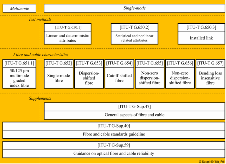
In the realm of telecommunications, the precision and reliability of optical fibers and cables are paramount. The International Telecommunication Union (ITU) plays a crucial role in this by providing a series of recommendations that serve as global standards. The ITU-T G.650.x and G.65x series of recommendations are especially significant for professionals in the field. In this article, we delve into these recommendations and their interrelationships, as illustrated in Figure 1 .

ITU-T G.650.x Series: Definitions and Test Methods

#opticalfiber

The ITU-T G.650.x series is foundational for understanding single-mode fibers and cables. ITU-T G.650.1 is the cornerstone, offering definitions and test methods for linear and deterministic parameters of single-mode fibers. This includes key measurements like attenuation and chromatic dispersion, which are critical for ensuring fiber performance over long distances.

Moving forward, ITU-T G.650.2 expands on the initial parameters by providing definitions and test methods for statistical and non-linear parameters. These are essential for predicting fiber behavior under varying signal powers and during different transmission phenomena.

For those involved in assessing installed fiber links, ITU-T G.650.3 offers valuable test methods. It’s tailored to the needs of field technicians and engineers who analyze the performance of installed single-mode fiber cable links, ensuring that they meet the necessary standards for data transmission.

ITU-T G.65x Series: Specifications for Fibers and Cables

The ITU-T G.65x series recommendations provide specifications for different types of optical fibers and cables. ITU-T G.651.1 targets the optical access network with specifications for 50/125 µm multimode fiber and cable, which are widely used in local area networks and data centers due to their ability to support high data rates over short distances.

The series then progresses through various single-mode fiber specifications:

  • ITU-T G.652: The standard single-mode fiber, suitable for a wide range of applications.
  • ITU-T G.653: Dispersion-shifted fibers optimized for minimizing chromatic dispersion.
  • ITU-T G.654: Features a cut-off shifted fiber, often used for submarine cable systems.
  • ITU-T G.655: Non-zero dispersion-shifted fibers, which are ideal for long-haul transmissions.
  • ITU-T G.656: Fibers designed for a broader range of wavelengths, expanding the capabilities of dense wavelength division multiplexing systems.
  • ITU-T G.657: Bending loss insensitive fibers, offering robust performance in tight bends and corners.

Historical Context and Current References

It’s noteworthy to mention that the multimode fiber test methods were initially described in ITU-T G.651. However, this recommendation was deleted in 2008, and now the test methods for multimode fibers are referenced in existing IEC documents. Professionals seeking current standards for multimode fiber testing should refer to these IEC documents for the latest guidelines.

Conclusion

The ITU-T recommendations play a critical role in the standardization and performance optimization of optical fibers and cables. By adhering to these standards, industry professionals can ensure compatibility, efficiency, and reliability in fiber optic networks. Whether you are a network designer, a field technician, or an optical fiber manufacturer, understanding these recommendations is crucial for maintaining the high standards expected in today’s telecommunication landscape.

Reference

https://www.itu.int/rec/T-REC-G/e