Tag

Telecommunications

Browsing

In this ever-evolving landscape of optical networking, the development of coherent optical standards, such as 400G ZR and ZR+, represents a significant leap forward in addressing the insatiable demand for bandwidth, efficiency, and scalability in data centers and network infrastructure. This technical blog delves into the nuances of these standards, comparing their features, applications, and how they are shaping the future of high-capacity networking.

Introduction to 400G ZR

The 400G ZR standard, defined by the Optical Internetworking Forum (OIF), is a pivotal development in the realm of optical networking, setting the stage for the next generation of data transmission over optical fiber’s. It is designed to facilitate the transfer of 400 Gigabit Ethernet over single-mode fiber across distances of up to 120 kilometers without the need for signal amplification or regeneration. This is achieved through the use of advanced modulation techniques like DP-16QAM and state-of-the-art forward error correction (FEC).

Key features of 400G ZR include:

  • High Capacity: Supports the transmission of 400 Gbps using a single wavelength.
  • Compact Form-Factor: Integrates into QSFP-DD and OSFP modules, aligning with industry standards for data center equipment.
  • Cost Efficiency: Reduces the need for external transponders and simplifies network architecture, lowering both CAPEX and OPEX.

Emergence of 400G ZR+

Building upon the foundation set by 400G ZR, the 400G ZR+ standard extends the capabilities of its predecessor by increasing the transmission reach and introducing flexibility in modulation schemes to cater to a broader range of network topologies and distances. The OpenZR+ MSA has been instrumental in this expansion, promoting interoperability and open standards in coherent optics.

Key enhancements in 400G ZR+ include:

  • Extended Reach: With advanced FEC and modulation, ZR+ can support links up to 2,000 km, making it suitable for longer metro, regional, and even long-haul deployments.
  • Versatile Modulation: Offers multiple configuration options (e.g., DP-16QAM, DP-8QAM, DP-QPSK), enabling operators to balance speed, reach, and optical performance.
  • Improved Power Efficiency: Despite its extended capabilities, ZR+ maintains a focus on energy efficiency, crucial for reducing the environmental impact of expanding network infrastructures.

ZR vs. ZR+: A Comparative Analysis

Feature. 400G ZR 400G ZR+
Reach Up to 120 km Up to 2,000 km
Modulation DP-16QAM DP-16QAM, DP-8QAM, DP-QPSK
Form Factor QSFP-DD, OSFP QSFP-DD, OSFP
Application Data center interconnects Metro, regional, long-haul

Adding few more interesting table for readersZR

The Future Outlook

The advent of 400G ZR and ZR+ is not just a technical upgrade; it’s a paradigm shift in how we approach optical networking. With these technologies, network operators can now deploy more flexible, efficient, and scalable networks, ready to meet the future demands of data transmission.

Moreover, the ongoing development and expected introduction of XR optics highlight the industry’s commitment to pushing the boundaries of what’s possible in optical networking. XR optics, with its promise of multipoint capabilities and aggregation of lower-speed interfaces, signifies the next frontier in coherent optical technology.

Optical Amplifiers (OAs) are key parts of today’s communication world. They help send data under the sea, land and even in space .In fact it is used in all electronic and telecommunications industry which has allowed human being develop and use gadgets and machines in daily routine.Due to OAs only; we are able to transmit data over a distance of few 100s too 1000s of kilometers.

Classification of OA Devices

Optical Amplifiers, integral in managing signal strength in fiber optics, are categorized based on their technology and application. These categories, as defined in ITU-T G.661, include Power Amplifiers (PAs), Pre-amplifiers, Line Amplifiers, OA Transmitter Subsystems (OATs), OA Receiver Subsystems (OARs), and Distributed Amplifiers.

amplifier

Scheme of insertion of an OA device

  1. Power Amplifiers (PAs): Positioned after the optical transmitter, PAs boost the signal power level. They are known for their high saturation power, making them ideal for strengthening outgoing signals.
  2. Pre-amplifiers: These are used before an optical receiver to enhance its sensitivity. Characterized by very low noise, they are crucial in improving signal reception.
  3. Line Amplifiers: Placed between passive fiber sections, Line Amplifiers are low noise OAs that extend the distance covered before signal regeneration is needed. They are particularly useful in point-multipoint connections in optical access networks.
  4. OA Transmitter Subsystems (OATs): An OAT integrates a power amplifier with an optical transmitter, resulting in a higher power transmitter.
  5. OA Receiver Subsystems (OARs): In OARs, a pre-amplifier is combined with an optical receiver, enhancing the receiver’s sensitivity.
  6. Distributed Amplifiers: These amplifiers, such as those using Raman pumping, provide amplification over an extended length of the optical fiber, distributing amplification across the transmission span.
Scheme of insertion of an OAT

Scheme of insertion of an OAT
Scheme of insertion of an OAR

Applications and Configurations

The application of these OA devices can vary. For instance, a Power Amplifier (PA) might include an optical filter to minimize noise or separate signals in multiwavelength applications. The configurations can range from simple setups like Tx + PA + Rx to more complex arrangements like Tx + BA + LA + PA + Rx, as illustrated in the various schematics provided in the IEC standards.

Building upon the foundational knowledge of Optical Amplifiers (OAs), it’s essential to understand the practical configurations of these devices in optical networks. According to the definitions of Booster Amplifiers (BAs), Pre-amplifiers (PAs), and Line Amplifiers (LAs), and referencing Figure 1 from the IEC standards, we can explore various OA device applications and their configurations. These setups illustrate how OAs are integrated into optical communication systems, each serving a unique purpose in enhancing signal integrity and network performance.

  1. Tx + BA + Rx Configuration: This setup involves a transmitter (Tx), followed by a Booster Amplifier (BA), and then a receiver (Rx). The BA is used right after the transmitter to increase the signal power before it enters the long stretch of the fiber. This configuration is particularly useful in long-haul communication systems where maintaining a strong signal over vast distances is crucial.
  2. Tx + PA + Rx Configuration: Here, the system comprises a transmitter, followed by a Pre-amplifier (PA), and then a receiver. The PA is positioned close to the receiver to improve its sensitivity and to amplify the weakened incoming signal. This setup is ideal for scenarios where the incoming signal strength is low, and enhanced detection is required.
  3. Tx + LA + Rx Configuration: In this configuration, a Line Amplifier (LA) is placed between the transmitter and receiver. The LA’s role is to amplify the signal partway through the transmission path, effectively extending the reach of the communication link. This setup is common in both long-haul and regional networks.
  4. Tx + BA + PA + Rx Configuration: This more complex setup involves both a BA and a PA, with the BA placed after the transmitter and the PA before the receiver. This combination allows for both an initial boost in signal strength and a final amplification to enhance receiver sensitivity, making it suitable for extremely long-distance transmissions or when signals pass through multiple network segments.
  5. Tx + BA + LA + Rx Configuration: Combining a BA and an LA provides a powerful solution for extended reach. The BA boosts the signal post-transmission, and the LA offers additional amplification along the transmission path. This configuration is particularly effective in long-haul networks with significant attenuation.
  6. Tx + LA + PA + Rx Configuration: Here, the LA is used for mid-path amplification, while the PA is employed near the receiver. This setup ensures that the signal is sufficiently amplified both during transmission and before reception, which is vital in networks with long spans and higher signal loss.
  7. Tx + BA + LA + PA + Rx Configuration: This comprehensive setup includes a BA, an LA, and a PA, offering a robust solution for maintaining signal integrity across very long distances and complex network architectures. The BA boosts the initial signal strength, the LA provides necessary mid-path amplification, and the PA ensures that the receiver can effectively detect the signal.

Characteristics of Optical Amplifiers

Each type of OA has specific characteristics that define its performance in different applications, whether single-channel or multichannel. These characteristics include input and output power ranges, wavelength bands, noise figures, reflectance, and maximum tolerable reflectance at input and output, among others.

For instance, in single-channel applications, a Power Amplifier’s characteristics would include an input power range, output power range, power wavelength band, and signal-spontaneous noise figure. In contrast, for multichannel applications, additional parameters like channel allocation, channel input and output power ranges, and channel signal-spontaneous noise figure become relevant.

Optically Amplified Transmitters and Receivers

In the realm of OA subsystems like OATs and OARs, the focus shifts to parameters like bit rate, application code, operating signal wavelength range, and output power range for transmitters, and sensitivity, overload, and bit error ratio for receivers. These parameters are critical in defining the performance and suitability of these subsystems for specific applications.

Understanding Through Practical Examples

To illustrate, consider a scenario in a long-distance fiber optic communication system. Here, a Line Amplifier might be employed to extend the transmission distance. This amplifier would need to have a low noise figure to minimize signal degradation and a high saturation output power to ensure the signal remains strong over long distances. The specific values for these parameters would depend on the system’s requirements, such as the total transmission distance and the number of channels being used.

Advanced Applications of Optical Amplifiers

  1. Long-Haul Communication: In long-haul fiber optic networks, Line Amplifiers (LAs) play a critical role. They are strategically placed at intervals to compensate for signal loss. For example, an LA with a high saturation output power of around +17 dBm and a low noise figure, typically less than 5 dB, can significantly extend the reach of the communication link without the need for electronic regeneration.
  2. Submarine Cables: Submarine communication cables, spanning thousands of kilometers, heavily rely on Distributed Amplifiers, like Raman amplifiers. These amplifiers uniquely boost the signal directly within the fiber, offering a more distributed amplification approach, which is crucial for such extensive undersea networks.
  3. Metropolitan Area Networks: In shorter, more congested networks like those in metropolitan areas, a combination of Booster Amplifiers (BAs) and Pre-amplifiers can be used. A BA, with an output power range of up to +23 dBm, can effectively launch a strong signal into the network, while a Pre-amplifier at the receiving end, with a very low noise figure (as low as 4 dB), enhances the receiver’s sensitivity to weak signals.
  4. Optical Add-Drop Multiplexers (OADMs): In systems using OADMs for channel multiplexing and demultiplexing, Line Amplifiers help in maintaining signal strength across the channels. The ability to handle multiple channels, each potentially with different power levels, is crucial. Here, the channel addition/removal (steady-state) gain response and transient gain response become significant parameters.

Technological Innovations and Challenges

The development of OA technologies is not without challenges. One of the primary concerns is managing the noise, especially in systems with multiple amplifiers. Each amplification stage adds some noise, quantified by the signal-spontaneous noise figure, which can accumulate and degrade the overall signal quality.

Another challenge is the management of Polarization Mode Dispersion (PMD) in Line Amplifiers. PMD can cause different light polarizations to travel at slightly different speeds, leading to signal distortion. Modern LAs are designed to minimize PMD, a critical parameter in high-speed networks.

Future of Optical Amplifiers in Industry

The future of OAs is closely tied to the advancements in fiber optic technology. As data demands continue to skyrocket, the need for more efficient, higher-capacity networks grows. Optical Amplifiers will continue to evolve, with research focusing on higher power outputs, broader wavelength ranges, and more sophisticated noise management techniques.

Innovations like hybrid amplification techniques, combining the benefits of Raman and Erbium-Doped Fiber Amplifiers (EDFAs), are on the horizon. These hybrid systems aim to provide higher performance, especially in terms of power efficiency and noise reduction.

References

ITU-T :https://www.itu.int/en/ITU-T/Pages/default.aspx

Image :https://www.chinacablesbuy.com/guide-to-optical-amplifier.html

Optical networks are the backbone of the internet, carrying vast amounts of data over great distances at the speed of light. However, maintaining signal quality over long fiber runs is a challenge due to a phenomenon known as noise concatenation. Let’s delve into how amplified spontaneous emission (ASE) noise affects Optical Signal-to-Noise Ratio (OSNR) and the performance of optical amplifier chains.

The Challenge of ASE Noise

ASE noise is an inherent byproduct of optical amplification, generated by the spontaneous emission of photons within an optical amplifier. As an optical signal traverses through a chain of amplifiers, ASE noise accumulates, degrading the OSNR with each subsequent amplifier in the chain. This degradation is a crucial consideration in designing long-haul optical transmission systems.

Understanding OSNR

OSNR measures the ratio of signal power to ASE noise power and is a critical parameter for assessing the performance of optical amplifiers. A high OSNR indicates a clean signal with low noise levels, which is vital for ensuring data integrity.

Reference System for OSNR Estimation

As depicted in Figure below), a typical multichannel N span system includes a booster amplifier, N−1 line amplifiers, and a preamplifier. To simplify the estimation of OSNR at the receiver’s input, we make a few assumptions:

Representation of optical line system interfaces (a multichannel N-span system)
  • All optical amplifiers, including the booster and preamplifier, have the same noise figure.
  • The losses of all spans are equal, and thus, the gain of the line amplifiers compensates exactly for the loss.
  • The output powers of the booster and line amplifiers are identical.

Estimating OSNR in a Cascaded System

E1: Master Equation For OSNR

E1: Master Equation For OSNR

Pout is the output power (per channel) of the booster and line amplifiers in dBm, L is the span loss in dB (which is assumed to be equal to the gain of the line amplifiers), GBA is the gain of the optical booster amplifier in dB, NFis the signal-spontaneous noise figure of the optical amplifier in dB, h is Planck’s constant (in mJ·s to be consistent with Pout in dBm), ν is the optical frequency in Hz, νr is the reference bandwidth in Hz (corresponding to c/Br ), N–1 is the total number of line amplifiers.

The OSNR at the receivers can be approximated by considering the output power of the amplifiers, the span loss, the gain of the optical booster amplifier, and the noise figure of the amplifiers. Using constants such as Planck’s constant and the optical frequency, we can derive an equation that sums the ASE noise contributions from all N+1 amplifiers in the chain.

Simplifying the Equation

Under certain conditions, the OSNR equation can be simplified. If the booster amplifier’s gain is similar to that of the line amplifiers, or if the span loss greatly exceeds the booster gain, the equation can be modified to reflect these scenarios. These simplifications help network designers estimate OSNR without complex calculations.

1)          If the gain of the booster amplifier is approximately the same as that of the line amplifiers, i.e., GBA » L, above Equation E1 can be simplified to:

osnr_2

E1-1

2)          The ASE noise from the booster amplifier can be ignored only if the span loss L (resp. the gain of the line amplifier) is much greater than the booster gain GBA. In this case Equation E1-1 can be simplified to:

E1-2

3)          Equation E1-1 is also valid in the case of a single span with only a booster amplifier, e.g., short‑haul multichannel IrDI in Figure 5-5 of [ITU-T G.959.1], in which case it can be modified to:

E1-3

4)          In case of a single span with only a preamplifier, Equation E1 can be modified to:

Practical Implications for Network Design

Understanding the accumulation of ASE noise and its impact on OSNR is crucial for designing reliable optical networks. It informs decisions on amplifier placement, the necessity of signal regeneration, and the overall system architecture. For instance, in a system where the span loss is significantly high, the impact of the booster amplifier on ASE noise may be negligible, allowing for a different design approach.

Conclusion

Noise concatenation is a critical factor in the design and operation of optical networks. By accurately estimating and managing OSNR, network operators can ensure signal quality, minimize error rates, and extend the reach of their optical networks.

In a landscape where data demands are ever-increasing, mastering the intricacies of noise concatenation and OSNR is essential for anyone involved in the design and deployment of optical communication systems.

References

https://www.itu.int/rec/T-REC-G/e

When we talk about the internet and data, what often comes to mind are the speeds and how quickly we can download or upload content. But behind the scenes, it’s a game of efficiently packing data signals onto light waves traveling through optical fibers.If you’re an aspiring telecommunications professional or a student diving into the world of fiber optics, understanding the allocation of spectral bands is crucial. It’s like knowing the different climates in a world map of data transmission. Let’s explore the significance of these bands as defined by ITU-T recommendations and what they mean for fiber systems.

#opticalband

The Role of Spectral Bands in Single-Mode Fiber Systems

Original O-Band (1260 – 1360 nm): The journey of fiber optics began with the O-band, chosen for ITU T G.652 fibers due to its favorable dispersion characteristics and alignment with the cut-off wavelength of the cable. This band laid the groundwork for optical transmission without the need for amplifiers, making it a cornerstone in the early days of passive optical networks.

Extended E-Band (1360 – 1460 nm): With advancements, the E-band emerged to accommodate the wavelength drift of uncooled lasers. This extended range allowed for greater flexibility in transmissions, akin to broadening the canvas on which network artists could paint their data streams.

Short Wavelength S-Band (1460 – 1530 nm): The S-band, filling the gap between the E and C bands, has historically been underused for data transmission. However, it plays a crucial role in supporting the network infrastructure by housing pump lasers and supervisory channels, making it the unsung hero of the optical spectrum.

Conventional C-Band (1530 – 1565 nm): The beloved C-band owes its popularity to the era of erbium-doped fiber amplifiers (EDFAs), which provided the necessary gain for dense wavelength division multiplexing (DWDM) systems. It’s the bread and butter of the industry, enabling vast data capacity and robust long-haul transmissions.

Long Wavelength L-Band (1565 – 1625 nm): As we seek to expand our data highways, the L-band has become increasingly important. With fiber performance improving over a range of temperatures, this band offers a wider wavelength range for signal transmission, potentially doubling the capacity when combined with the C-band.

Ultra-Long Wavelength U-Band (1625 – 1675 nm): The U-band is designated mainly for maintenance purposes and is not currently intended for transmitting traffic-bearing signals. This band ensures the network’s longevity and integrity, providing a dedicated spectrum for testing and monitoring without disturbing active data channels.

Historical Context and Technological Progress

It’s fascinating to explore why we have bands at all. The ITU G-series documents paint a rich history of fiber deployment, tracing the evolution from the first multimode fibers to the sophisticated single-mode fibers we use today.

In the late 1970s, multimode fibers were limited by both high attenuation at the 850 nm wavelength and modal dispersion. A leap to 1300 nm in the early 1980s marked a significant drop in attenuation and the advent of single-mode fibers. By the late 1980s, single-mode fibers were achieving commercial transmission rates of up to 1.7 Gb/s, a stark contrast to the multimode fibers of the past.

The designation of bands was a natural progression as single-mode fibers were designed with specific cutoff wavelengths to avoid modal dispersion and to capitalize on the low attenuation properties of the fiber.

The Future Beckons

With the ITU T G.65x series recommendations setting the stage, we anticipate future applications utilizing the full spectrum from 1260 nm to 1625 nm. This evolution, coupled with the development of new amplification technologies like thulium-doped amplifiers or Raman amplification, suggests that the S-band could soon be as important as the C and L bands.

Imagine a future where the combination of S+C+L bands could triple the capacity of our fiber infrastructure. This isn’t just a dream; it’s a realistic projection of where the industry is headed.

Conclusion

The spectral bands in fiber optics are not just arbitrary divisions; they’re the result of decades of research, development, and innovation. As we look to the horizon, the possibilities are as wide as the spectrum itself, promising to keep pace with our ever-growing data needs.

Reference

https://www.itu.int/rec/T-REC-G/e

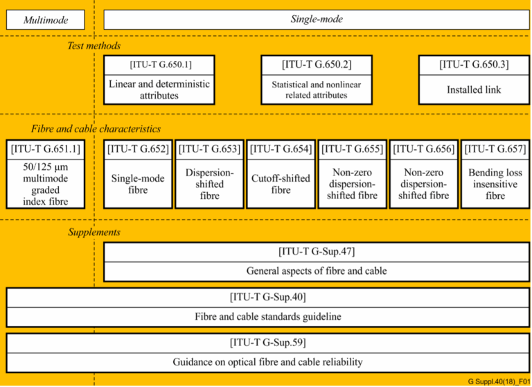
In the realm of telecommunications, the precision and reliability of optical fibers and cables are paramount. The International Telecommunication Union (ITU) plays a crucial role in this by providing a series of recommendations that serve as global standards. The ITU-T G.650.x and G.65x series of recommendations are especially significant for professionals in the field. In this article, we delve into these recommendations and their interrelationships, as illustrated in Figure 1 .

ITU-T G.650.x Series: Definitions and Test Methods

#opticalfiber

The ITU-T G.650.x series is foundational for understanding single-mode fibers and cables. ITU-T G.650.1 is the cornerstone, offering definitions and test methods for linear and deterministic parameters of single-mode fibers. This includes key measurements like attenuation and chromatic dispersion, which are critical for ensuring fiber performance over long distances.

Moving forward, ITU-T G.650.2 expands on the initial parameters by providing definitions and test methods for statistical and non-linear parameters. These are essential for predicting fiber behavior under varying signal powers and during different transmission phenomena.

For those involved in assessing installed fiber links, ITU-T G.650.3 offers valuable test methods. It’s tailored to the needs of field technicians and engineers who analyze the performance of installed single-mode fiber cable links, ensuring that they meet the necessary standards for data transmission.

ITU-T G.65x Series: Specifications for Fibers and Cables

The ITU-T G.65x series recommendations provide specifications for different types of optical fibers and cables. ITU-T G.651.1 targets the optical access network with specifications for 50/125 µm multimode fiber and cable, which are widely used in local area networks and data centers due to their ability to support high data rates over short distances.

The series then progresses through various single-mode fiber specifications:

  • ITU-T G.652: The standard single-mode fiber, suitable for a wide range of applications.
  • ITU-T G.653: Dispersion-shifted fibers optimized for minimizing chromatic dispersion.
  • ITU-T G.654: Features a cut-off shifted fiber, often used for submarine cable systems.
  • ITU-T G.655: Non-zero dispersion-shifted fibers, which are ideal for long-haul transmissions.
  • ITU-T G.656: Fibers designed for a broader range of wavelengths, expanding the capabilities of dense wavelength division multiplexing systems.
  • ITU-T G.657: Bending loss insensitive fibers, offering robust performance in tight bends and corners.

Historical Context and Current References

It’s noteworthy to mention that the multimode fiber test methods were initially described in ITU-T G.651. However, this recommendation was deleted in 2008, and now the test methods for multimode fibers are referenced in existing IEC documents. Professionals seeking current standards for multimode fiber testing should refer to these IEC documents for the latest guidelines.

Conclusion

The ITU-T recommendations play a critical role in the standardization and performance optimization of optical fibers and cables. By adhering to these standards, industry professionals can ensure compatibility, efficiency, and reliability in fiber optic networks. Whether you are a network designer, a field technician, or an optical fiber manufacturer, understanding these recommendations is crucial for maintaining the high standards expected in today’s telecommunication landscape.

Reference

https://www.itu.int/rec/T-REC-G/e

Carrier Ethernet: A Formal Definition

The MEF (Metro Ethernet Forum)  has defined Carrier Ethernet as the “ubiquitous, standardized, Carrier-class service defined by five attributes that distinguish Carrier Ethernet from the familiar LAN based Ethernet.” As depicted in Figure , these five attributes, in no particular order, are

1. Standardized services  

•E-Line, E-LAN provide transparent, private line, virtual private line and LAN services
•A ubiquitous service providing globally & locally via standardized equipment
•Requires no changes to customer LAN equipment or networks and accommodates existing network connectivity such as, time-sensitive, TDM traffic and signaling
•Ideally suited to converged voice, video & data networks
•Wide choice and granularity of bandwidth and quality of service options

  2. Scalability

•The ability for millions to use a network service that is ideal for the widest variety of business, information, communications and entertainment applications with voice, video and data
•Spans Access & Metro to National & Global Services over a wide variety of physical infrastructures implemented by a wide range of Service Providers
•Scalability of bandwidth from 1Mbps to 10Gbps and beyond, in granular increments


3. Reliability

•The ability for the network to detect & recover from incidents without impacting users
•Meeting the most demanding quality and availability requirements
•Rapid recovery time when problems do occur, as low as 50ms

4. Quality of Service (QoS)

•Wide choice and granularity of bandwidth and quality of service options
•Service Level Agreements (SLAs) that deliver end-to-end performance matching the requirements for voice, video and data over converged business and residential networks
•Provisioning via SLAs  that provide end-to-end performance based on CIR, frame loss, delay and delay variation characteristics

5. Service management

•The ability to monitor, diagnose and centrally manage the network, using standards-based vendor independent implementations
•Carrier-class OAM
•Rapid service provisioning


What is Carrier Ethernet?

Carrier Ethernet essentially augments traditional Ethernet, optimized for LAN deployment,with Carrier-class capabilities which make it optimal for deployment in Service Provider Access/Metro Area Networks and beyond, to the Wide Area Network. And conversely,from an end-user (enterprise) standpoint, Carrier Ethernet is a service that not only provides a standard Ethernet (or for that matter, a standardized non-Ethernethand-off  but also provides the robustness, deterministic performance, management, and flexibility expected of Carrier-class services.

Carrier Ethernet Architecture


Data moves from UNI to UNI across “the network” with a layered architecture.

When traffic moves between ETH domains is does so at the TRAN layer. This allows  Carrier Ethernet traffic to be
agnostic to the networks that it traverses

ce


ce1

MEF Carrier Ethernet Terminology

•The User Network Interface (UNI)
–The UNI is always provided by the Service Provider
–The UNI in a Carrier Ethernet Network is a physical Ethernet Interface at operating speeds 10Mbs, 100Mbps, 1Gbps or 10Gbps
•Ethernet Virtual Connection (EVC)
–Service container
–Connects two or more subscriber sites (UNI’s)
–An association of two or more UNIs
–Prevents data transfer between sites that are not part of the same EVC
–Three types of EVCs
•Point-to-Point
•Multipoint-to-Multipoint
•Rooted Multipoint
–Can be bundled or multiplexed on the same UNI
–Defined in MEF 10.2 technical specification
Carrier Ethernet Terminology
•UNI Type I
–A UNI compliant with MEF 13
–Manually Configurable
•UNI Type II
–Supports E-Tree
–Support service OAM, link protection
–Automatically Configurable via E-LMI
–Manageable via OAM
•Network to Network Interface (NNI)
–Network to Network Interface between distinct MEN operated by one or more carriers
–An active project of the MEF
•Metro Ethernet Network (MEN)
–An Ethernet transport network connecting user end-points
(Expanded to Access and Global networks in addition to the original Metro Network meaning)

Carrier Ethernet Service Types

ce3
Services Using E-Line Service Type

Ethernet Private Line (EPL)

•Replaces a TDM Private line
•Port-based service with single service (EVC) across dedicated UNIs providing site-to-site connectivity
•Typically delivered over SDH (Ethernet over SDH)
•Most popular Ethernet service due to its simplicity

Ethernet Virtual Private Line (EVPL)

•Replaces Frame Relay or ATM L2 VPN services
–To deliver higher bandwidth, end-to-end services
•Enables multiple services (EVCs) to be delivered over  single physical connection (UNI) to customer premises
•Supports “hub & spoke” connectivity via Service Multiplexed UNI at hub site
–Similar to Frame Relay or Private Line hub and spoke deployments
Services Using E-LAN Service Type
•EP-LAN: Each UNI dedicated to the EP-LAN service. Example use is Transparent LAN
•EVP-LAN: Service Multiplexing allowed at each UNI. Example use is Internet access and corporate VPN via one UNI

Services Using E-Tree Service Type

EP-Tree and EVP-Tree:  Both allow root – root and root – leaf communication but not leaf – leaf communication.

•EP-Tree requires dedication of the UNIs to the single EP-Tree service
•EVP-Tree allows each UNI to be support multiple simultaneous services at the cost of more complex configuration that EP-Tree

APPLICATION OF CARRIER ETHERNET


The Standardization of Services: Approved MEF Specifications

•MEF 2   Requirements and Framework for Ethernet Service Protection
•MEF 3  Circuit Emulation Service Definitions, Framework and Requirements in Metro Ethernet Networks
•MEF 4   Metro Ethernet Network Architecture Framework
Part 1: Generic Framework
•MEF 6  Metro Ethernet Services Definitions Phase I
•MEF 7   EMS-NMS Information Model
•MEF 8  Implementation Agreement for the Emulation of PDH Circuits over Metro Ethernet Networks
•MEF 9   Abstract Test Suite for Ethernet Services at the UNI
•MEF 10   Ethernet Services Attributes Phase I
•MEF 11   User Network Interface (UNI) Requirements and Framework
•MEF 12  Metro Ethernet Network Architecture Framework
Part 2: Ethernet Services Layer
•MEF 13   User Network Interface (UNI) Type 1 Implementation Agreement
•MEF 14   Abstract Test Suite for Traffic Management Phase 1
•MEF 15  Requirements for Management of Metro Ethernet
Phase 1 Network Elements
•MEF 16   Ethernet Local Management Interface

How the MEF Specifications Enable Carrier Ethernet