

Generic selectors
Exact matches only
Search in title
Search in content
Post Type Selectors
Articles
lp_course
lp_lesson
Back
HomeAnalysis800G and 1.6T for Hyperscale AI:Latency, Density, and Design Constraints
800G and 1.6T for Hyperscale AI:Latency, Density, and Design Constraints

800G and 1.6T for Hyperscale AI:Latency, Density, and Design Constraints

Last Updated: April 2, 2026
8 min read
92
800G and 1.6T for Hyperscale AI: Latency, Density, and Design Constraints
800G and 1.6T for Hyperscale AI:Latency, Density, and Design Constraints - Image 1

800G and 1.6T for Hyperscale AI:
Latency, Density, and Design Constraints

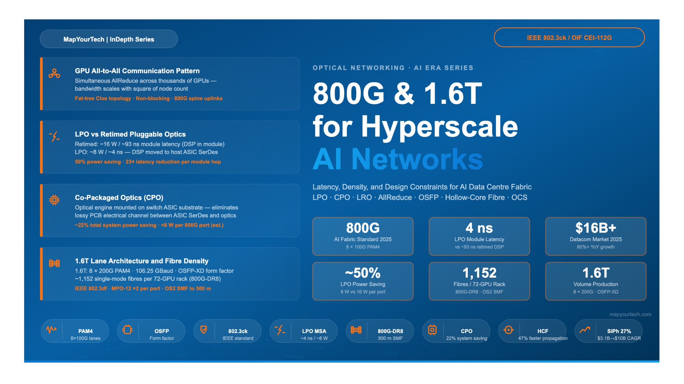
How all-to-all GPU communication patterns, sub-microsecond latency targets, and extreme power density requirements are reshaping optical interconnect design in hyperscale AI infrastructure.

Section 1

Introduction

The shift from conventional cloud computing to large-scale AI training has altered almost every dimension of data centre network design. Where traditional workloads generated predictable, north-south traffic flows between users and servers, AI training clusters create a fundamentally different pattern: dense, synchronised, east-west communication between thousands of GPU accelerators that must collectively function as a single logical compute engine. This traffic pattern — often called all-to-all communication — demands bandwidth, latency, and reliability characteristics that push optical interconnect technology to its limits.

The response from the industry has been a rapid transition through optical port speeds. The 400G generation, which was considered advanced three years ago, is now the baseline access tier for AI data centres. The 800G generation — based on eight lanes of 100 Gb/s each — has become the standard for AI fabric buildouts in 2025, with deployments doubling year-over-year. The 1.6T generation, leveraging 200 Gb/s per-lane technology, is entering early volume production and is already specified in hyperscale procurement contracts for the next infrastructure cycle.

This article covers the engineering rationale behind these transitions — the traffic patterns that demand them, the optical and electrical technologies that enable them, the latency constraints that shape them, and the power and density challenges that complicate them. It examines where pluggable optics remain the practical choice, where Linear Pluggable Optics (LPO) and its asymmetric variant Linear Receive Optics (LRO) offer compelling improvements, and where Co-Packaged Optics (CPO) become the preferred path. It also covers emerging fibre technologies — hollow-core and multi-core fibres — and optical circuit switching, all of which are shaping the next phase of AI cluster design.

Scope

This reference covers intra-data-centre optical interconnects for AI training and inference clusters, including the switch fabric, top-of-rack, and server attachment layers. Data centre interconnect coherent optics, metro transport, and submarine systems are outside scope. Forward-looking sections on emerging fibre and switching technologies are clearly labelled as such.

Section 2

2. AI Traffic Patterns and Why They Demand New Interconnect Designs

2.1 The All-to-All Communication Pattern

Training a large-scale AI model requires distributing computation across hundreds or thousands of GPU accelerators simultaneously. The work is split in several ways — across training data (data parallelism), across model layers (pipeline parallelism), and across the weights within a layer (tensor parallelism). Each parallelism strategy produces a specific communication pattern, and in combination they create demand for high-bandwidth, low-latency collective communication operations such as AllReduce, AllGather, and ReduceScatter.

An AllReduce operation requires every accelerator in a training group to share its locally computed gradient updates with all other accelerators in the group, aggregate the results, and distribute the aggregated result back to every accelerator — all before the next training step begins. In a cluster of thousands of GPUs, this generates a simultaneous, bidirectional, many-to-many traffic burst that is wholly unlike web traffic, database queries, or file I/O. It is a synchronised collective operation, meaning the fastest accelerator can only advance as fast as the slowest interconnect allows.

2.2 The Scale-Up and Scale-Out Network Layers

Modern AI cluster networks are organised into two physically distinct layers. The scale-up network connects GPU accelerators within a single server or a tightly coupled node group at the highest possible bandwidth and lowest latency. This layer uses specialised chip-to-chip interconnects, PCIe, or CXL switches, and is internal to the compute node — transparent to the Ethernet fabric.

The scale-out network (also called the backend AI fabric) connects compute nodes across the cluster. This is where 800G and 1.6T optical transceivers are deployed. It must carry collective communication traffic with near-zero congestion, provide a non-blocking topology, and deliver end-to-end latency that keeps collective operations within the compute step window.

AI Data Centre Network Architecture — Scale-Up, Scale-Out, and Frontend Networks Cloud / WAN Backbone Internet · Storage Services · Users Super-Spine — Frontend Network 51.2 Tbps ASIC · 800G uplinks to Cloud · 1.6T planned FRONTEND User-facing traffic Spine Switch A 25.6 Tbps · 800G ports Spine Switch B 25.6 Tbps · 800G ports Spine Switch C 25.6 Tbps · 800G ports BACKEND SCALE-OUT AllReduce traffic ToR Switch 1 800G up · 400G down ToR Switch 2 800G up · 400G down ToR Switch 3 800G up · 400G down ToR Switch 4 800G up · 400G down AI Accelerator Rack 1 GPU × 8 GPU × 8 GPU × 8 GPU × 8 NIC · CPU · PCIe/CXL Scale-Up (NVLink/UALink) Scale-Out NICs → ToR 400G per accelerator port AI Accelerator Rack 2 GPU × 8 GPU × 8 GPU × 8 GPU × 8 NIC · CPU · PCIe/CXL Scale-Up (NVLink/UALink) Scale-Out NICs → ToR 400G per accelerator port AI Accelerator Rack 3 GPU × 8 GPU × 8 GPU × 8 GPU × 8 NIC · CPU · PCIe/CXL Scale-Up (NVLink/UALink) Scale-Out NICs → ToR 400G per accelerator port AI Accelerator Rack 4 GPU × 8 GPU × 8 GPU × 8 GPU × 8 NIC · CPU · PCIe/CXL Scale-Up (NVLink/UALink) Scale-Out NICs → ToR 400G per accelerator port Network Layer Summary Scale-Up (golden arrows) Within-server GPU interconnect NVLink / UALink / PCIe / CXL Transparent to Ethernet fabric Scale-Out (green arrows) Rack-to-rack · ToR + Spine 800G optics deployed here PRIMARY 800G/1.6T domain Frontend (blue arrows) Super-Spine → Cloud User / storage traffic Scale-Up interconnect (gold) is internal to each server; Scale-Out (green) spans racks via ToR and Spine at 800G. The Frontend (purple/blue) carries orchestration and user traffic to the cloud backbone, separate from the AI training fabric.
Figure: AI Data Centre Network Architecture — Scale-Up Network (within-server GPU fabric via NVLink/UALink/PCIe, shown in gold), Scale-Out Backend Network (rack-to-rack via ToR and Spine at 800G, in green), and Frontend Network (cluster-to-cloud via Super-Spine). The scale-out layer is where 800G and 1.6T optical transceivers are deployed.

2.3 Rail Architecture for AllReduce Efficiency

A rail architecture groups GPU servers so that each GPU within a server connects to a different spine switch through dedicated top-of-rack (ToR) switches on separate rails. In a single-rail design, all GPU ports from a server route through one ToR. In a multi-rail design, GPU ports are distributed across multiple ToR switches, each connected to different spine switches.

Multi-rail architectures reduce AllReduce congestion because traffic from different GPUs within the same server exits through different uplinks, reducing the probability that synchronisation traffic from multiple GPUs contends for the same spine links simultaneously. The optical design implication is that each rack requires multiple ToR switches with 800G uplinks, increasing total fibre count and switch port count per rack — a direct planning input for fabric sizing and cabling infrastructure.

2.4 Why East-West Traffic Dominates

In AI training clusters, the dominant pattern is server-to-server (east-west) gradient synchronisation traffic. In a cluster with thousands of GPU accelerators, a single training step may require each node to transmit its full gradient update to every other node simultaneously — meaning aggregate east-west bandwidth scales with the square of the number of nodes, while north-south traffic scales only linearly. This structural difference is why AI data centres invest in switch silicon with dramatically higher port counts, and why the ratio of optical transceivers to GPU accelerators has increased substantially compared to traditional cloud deployments.

Figure 1: AI Data Centre Fabric Architecture — Scale-Up and Scale-Out Layers SUPER-SPINE 1.6T links planned (Frontend) SPINE 800G uplinks (Backend fabric) LEAF / TOR 400G / 800G downlinks GPU SERVER Scale-up network (NVLink / high-bw fabric) Internal to node Super-Spine 151.2T ASIC Super-Spine 251.2T ASIC Super-Spine 351.2T ASIC Super-Spine 451.2T ASIC Spine A25.6T ASIC Spine B25.6T ASIC Spine C25.6T ASIC Spine D25.6T ASIC TOR / Leaf 1800G uplinks TOR / Leaf 2800G uplinks TOR / Leaf 3800G uplinks TOR / Leaf 4800G uplinks GPU Rack 1 GPU GPU GPU GPU GPU GPU 400G downlinks GPU Rack 2 GPU GPU GPU GPU GPU GPU 400G downlinks GPU Rack 3 GPU GPU GPU GPU GPU GPU 400G downlinks GPU Rack 4 GPU GPU GPU GPU GPU GPU 400G downlinks 800G links All-to-All All-to-All All-to-All 1.6T planned 1.6T planned 1.6T planned 1.6T planned 800G links Key Design Factors Scale-Out Fabric 800G OSFP at spine and TOR uplinks Non-blocking Clos Fat-tree topology prevents congestion Latency Target End-to-end <10 µs LPO saves ~712 ns RTT Fibre per Rack ~1,152 fibres for 72 GPU rack (800G-DR8) ASIC Bandwidth 6.4 → 12.8 → 25.6 → 51.2 Tbps Traffic Pattern East-West dominates AllReduce / AllGather ReduceScatter ops Scale-up connections (within server) not shown. Backend fabric carries AI collective operations across racks.
Figure 1: AI Data Centre Fabric Architecture — Super-Spine, Spine, Leaf/TOR, and GPU Rack layers showing link speeds, all-to-all communication pattern, and key design factors per tier.
Section 3

3. Foundational Concepts: 800G and 1.6T Optical Technology

3.1 Lane Architecture and Modulation

The progression from 400G to 800G to 1.6T in intra-data-centre optics follows a consistent pattern: the industry increases speed either by increasing the number of lanes at a fixed lane rate, or by increasing the per-lane data rate while keeping the lane count fixed, or both. For short-reach intra-data-centre applications, direct-detection with four-level Pulse Amplitude Modulation (PAM4) is the dominant modulation scheme. PAM4 encodes 2 bits per symbol, doubling the data rate compared to non-return-to-zero (NRZ) signalling at the same baud rate — at the cost of reduced noise margin that makes Forward Error Correction (FEC) mandatory.

Premium Article — Free 20% Preview

Read the Full Analysis with Premium

The remaining 80% of this article — the design numbers, trade-offs and field guidance — is part of MapYourTech Premium, along with the full premium library, courses and professional tools.


Instant access · Cancel anytime · 48-hour trial available
Sanjay Yadav

Optical Communications & Network Automation Expert | Author of 3 Books for Optical Engineers | Founder, MapYourTech

Optical networking engineer with nearly two decades of experience across DWDM, OTN, coherent optics, submarine systems, and cloud infrastructure. Founder of MapYourTech.

Follow on LinkedIn

You May Also Like

52 min read 12 0 Like The Submarine Cable Stack: Open Cables, GSNR, SDM and Power Skip to main content...
  • Free
  • July 10, 2026
32 min read 10 0 Like Coherent DSP Architecture: From ADC Samples to Client Bits MAPYOURTECH | COHERENT OPTICS DEEP...
  • Free
  • July 10, 2026
42 min read 14 0 Like Building an Optical NOC Dashboard with OpenConfig Telemetry Skip to main content MapYourTech |...
  • Free
  • July 10, 2026

Course Title

Course description and key highlights

Course Content

Course Details
