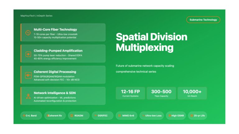
Spatial Division Multiplexing: Future of Submarine Network Capacity Spatial Division Multiplexing: Future of Submarine Network Capacity Exploring the Next Generation...
Multi-Vendor ROADM Interoperability – Part 1: Introduction & Architecture Multi-Vendor ROADM Interoperability in Optical Transport Networks Introduction The optical networking...
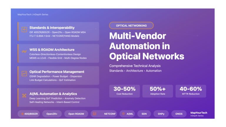
Multi-Vendor Integration in Optical Networks: A Comprehensive Technical Analysis Multi-Vendor Automation in Optical Networks: A Comprehensive Technical Analysis Introduction The...
Multi-Vendor WSS Integration in Optical Line Systems: Comprehensive Technical Guide Multi-Vendor WSS Integration in Optical Line Systems Comprehensive Technical Guide:...