
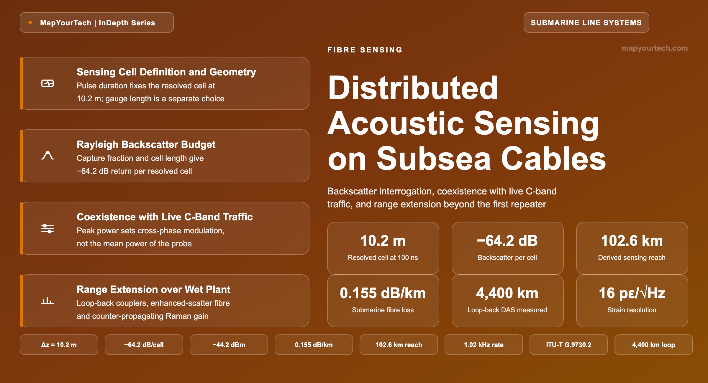
Distributed Acoustic Sensing over Operational Submarine Cables
Backscatter interrogation resolves strain to ten metres and runs out of optical budget near 100 km; this reference derives that limit and sets out the dark fibre, coexistence and multi-span choices that follow from it.
An instrument describes what it can attribute and nothing beyond that.
What You Will Learn
- Define the resolved sensing cell from pulse duration and derive the 10.2 m cell used throughout this article (Section 2, Fig. 1).
- Separate resolved cell length, gauge length and channel spacing, and state which of the three follows from pulse duration alone.
- Build the Rayleigh backscatter budget that places the demodulation threshold at −76 dBm and the reach at 103 km (Section 5, Chart 1).
- Quantify why halving the cell to 5.1 m costs 19 km of reach, and why a 10× averaging gain buys only 32 km.
- Place the sensing probe against live C-band traffic under the no-net-impact requirement of ITU-T G.9730.2 (Section 6, Table 3).
- Select between a dedicated dark fibre, a shared live fibre and a repeater loop-back path using the decision flow of Fig. 4.
- Compare DAS against polarization, interferometric and SMART repeater sensing on range, resolution and wet plant impact (Section 10).
- Read the reach records that now stand at 200.6 km unrepeatered and 4,400 km multi-span, and what each one required.
1. Introduction
A submarine cable carries its own instrument. Every kilometre of installed fibre scatters a fraction of the light passing through it back toward the launch end, and the phase of that returning light changes when the fibre stretches. Interrogating that return turns a telecommunications asset into a strain array with tens of thousands of channels, at no cost in wet plant hardware and with no change to the cable already on the seabed. Distributed acoustic sensing (DAS) is the technique that reads it, and over the last five years it has recorded anchor drags, trawl gear, ship transits, whale vocalisations, ocean swell and megathrust earthquakes from cables that were laid to carry traffic and nothing else.
The constraint is optical budget. Rayleigh backscatter from a 100 ns probe pulse returns about 64 dB below the launched peak power, and it then pays fibre attenuation twice, once outbound and once on the return. On ultra-low-loss submarine fibre at 0.155 dB/km that round trip removes 31 dB per 100 km, and a coherent receiver operating close to the quantum limit runs out of usable phase signal shortly after. The 100 km figure that appears in every DAS datasheet is not a marketing round number; it is where the backscatter curve crosses the demodulation threshold, and Section 5 derives it from the fibre parameters and receiver bandwidth rather than quoting it.
Two further constraints follow from the plant rather than the physics. Submarine repeaters contain optical isolators, so backscatter generated in span two cannot propagate back through repeater one to reach the interrogator: a conventional DAS interrogator on a repeatered cable sees the first span and nothing else, however good its receiver. And the sensing probe has to share the cable with revenue traffic, which fixes what launch power, wavelength and waveform are admissible. ITU-T G.9730.2 states the requirement plainly for cable systems with sensing functions: adding sensing capability shall have no net impact on the telecommunication performance of the system, with any power budget allocation identified and measured at commissioning [standard-specified, ITU-T G.9730.2].
This article treats the interrogation chain from the resolved cell up to the whole-cable architectures, for unrepeatered festoon segments and for repeatered trunk systems. It covers the sensing cell derivation, the backscatter and receiver budget, the coexistence rules for in-band probing alongside live C-band channels, dark fibre provisioning, the range extension mechanisms and what each one costs, the performance parameters worth monitoring, a fault reference, and where DAS sits against polarization sensing, interferometric span arrays and instrumented SMART repeaters. Every number carries its evidence class in the sentence that states it. The boundary of the treatment is the optical layer: seismological inversion, machine learning classifiers and data pipeline design are named where they set an optical requirement and are otherwise left alone.
2. Sensing Cell Definition and Geometry
Distributed acoustic sensing is the measurement of dynamic longitudinal strain along an optical fibre by tracking the optical phase of coherent Rayleigh backscatter returned from successive positions in that fibre. The fibre reports strain in microstrain or in strain rate per second, resolved into contiguous cells whose length follows from the probe pulse duration, and sampled at the pulse repetition rate.
The quantity that governs every other design choice is the resolved sensing cell. A probe pulse of duration τ occupies a physical length Lp = c τ / ng in the fibre, but backscatter arriving at the receiver at any one instant was generated across only half that length, because light returning from the far edge of the pulse footprint has travelled the extra distance twice. The resolved cell is therefore half the pulse length, and no processing recovers detail finer than it.
Read the Full Analysis with Premium
The remaining 88% of this article — the design numbers, trade-offs and field guidance — is part of MapYourTech Premium, along with the full premium library, courses and professional tools.
You May Also Like
-
Free
-
August 22, 2026
-
Premium
-
August 22, 2026
-
Premium
-
August 22, 2026