
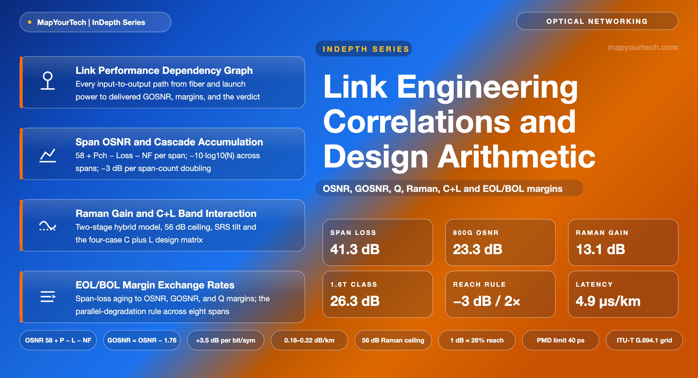
DWDM Link Engineering Correlations and Design Arithmetic for Architecture Decisions
Every feasibility question in optical transport reduces to a short chain of coupled quantities: span loss sets the optical signal-to-noise ratio (OSNR), launch power trades OSNR against nonlinear noise, the generalized OSNR (GOSNR) sets the Q-factor and the bit error rate before forward error correction (pre-FEC BER), and the end-of-life to beginning-of-life (EOL–BOL) gap decides whether the design survives its service life. This guide maps the full dependency graph, states the governing formulas with worked numbers from planning-tool simulations of a deployed long-haul core route, and compresses them into sensitivity rules an architect can run without a calculator.
What you can measure, you can improve.
Introduction
An optical architect reviewing a route rarely has time to run a full simulation before a design conversation. The useful skill is different: knowing which parameters drive which outcomes, by how much per unit, and where each relationship stops holding. This article assembles that knowledge as a single dependency framework covering fiber attenuation and type, span loss and its margin, amplifier noise figure and saturation power, Raman gain, launch-power optimization, Stimulated Raman Scattering (SRS) between bands, Optical Signal-to-Noise Ratio (OSNR), Generalized OSNR (GOSNR), Q-factor, pre-Forward-Error-Correction (FEC) Bit Error Rate (BER), chromatic dispersion (CD), polarization mode dispersion (PMD), polarization dependent loss (PDL), latency, and the End-of-Life (EOL) versus Beginning-of-Life (BOL) margins that connect all of them to service lifetime.
Three evidence classes appear throughout, and each number is labeled with its class where it is stated. Planning-tool simulation values come from link-engineering and power-budget exports for a deployed national core route, including one 172 km span with 40.2 dB of measured loss carrying 800 Gb/s at 138 GBd; these are the calibration anchors. Vendor design-rule values come from one optical vendor's planning-rule library (module OSNR thresholds, nonlinear coefficients per fiber type, launch-power and tilt equations); these are vendor calibrations, valid for that equipment family and representative of the industry pattern. Standard-specified and theoretical values (the −58 dBm quantum-noise constant, 10·log10 arithmetic, the Gaussian Noise model structure, ITU-T fiber classes) are general. The result is a set of correlations an architect can trust because each one is either derived from physics or reproduced against a simulator to within a tenth of a decibel.
This article is written for readers who take network design and simulation seriously and want the reference values at hand: the formulas, thresholds, and exchange rates are laid out for repeated consultation rather than a single read, and Table 10 gathers them into one starting sheet at the end.
The Link Performance Dependency Chain
Link engineering has a directed structure: three families of inputs feed two intermediate quantities, those feed three noise mechanisms, and the noise mechanisms combine into one delivered figure of merit that is compared against one required figure of merit. Everything else (Q-factor, BER, alarms, PASS/FAIL verdicts) is a re-expression of that comparison. Figure 1 draws the full graph.
The fiber plant contributes the attenuation coefficient α (dB/km), length, splice count, effective-area class (which sets the nonlinear factor β and the SRS factor R), the PMD coefficient, and dispersion D. The line equipment contributes Erbium-Doped Fiber Amplifier (EDFA) noise figure (NF) and saturation power Psat, Raman on/off gain and effective NF, and the insertion losses of Reconfigurable Optical Add-Drop Multiplexer (ROADM) and filter elements. The service mix contributes symbol rate Rs, bits per symbol, channel count Nch, channel spacing Δf, and FEC generation. Span loss and launch power are the two derived hinge quantities: almost every downstream correlation routes through one of them.
Two properties of this graph do most of the explanatory work. First, noise contributions combine as parallel sums in linear units (1/SNRtotal = Σ 1/SNRi), which means the worst contributor dominates and improvements to already-good contributors change almost nothing. Second, the two hinge quantities pull in opposite directions: raising launch power improves the ASE-limited OSNR at 1 dB per dB but degrades the nonlinear SNR at 2 dB per dB, which is why an optimum exists and why the sections below keep returning to it.
Read the Full Analysis with Premium
The remaining 88% of this article — the design numbers, trade-offs and field guidance — is part of MapYourTech Premium, along with the full premium library, courses and professional tools.
You May Also Like

-
Premium
-
August 18, 2026
-
Free
-
August 18, 2026

-
Free
-
August 18, 2026