
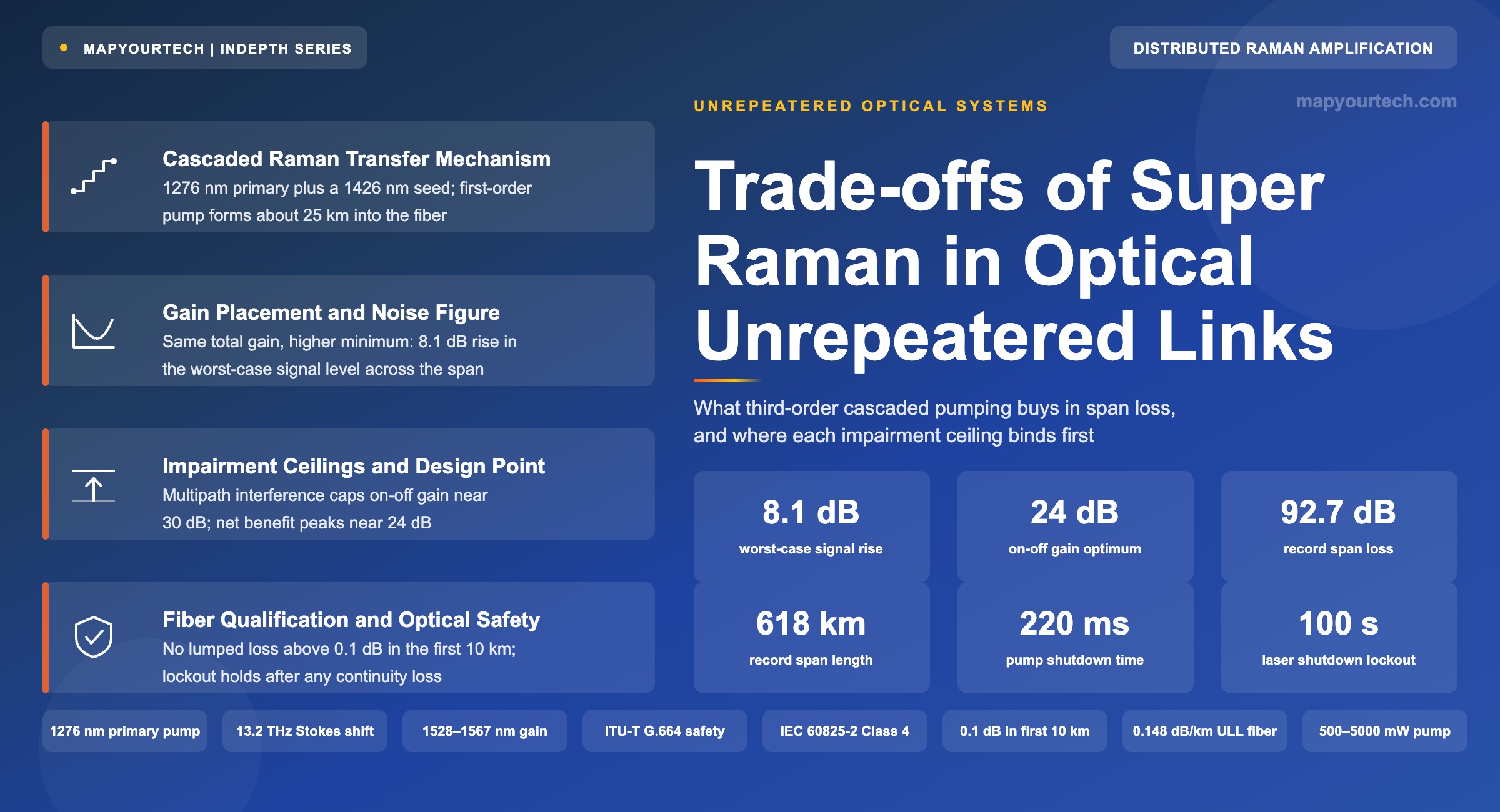
Trade-offs of Super Raman in Optical Unrepeatered Links
What third-order cascaded pumping buys in span loss, what it costs in Rayleigh noise, qualification effort and restoration time, and where each boundary sits.
Light brings us the news of the Universe
1. Introduction
An unrepeatered link places every active component on dry land. Between the two terminal stations there is nothing but glass, splice closures and, in the subsea case, armour and burial — no power feed, no submerged erbium, no branching electronics. That constraint is what makes the architecture attractive for island interconnection, coastal festoon routes, fjord and strait crossings, and offshore platform backhaul, where a repeatered wet plant would be sized for a fraction of its capability and would still carry the cost of a power feed equipment bay, a repeater qualification programme and a 25-year submerged reliability case. It is also what makes the architecture hard: the entire loss of a 300–600 km fiber path has to be recovered by equipment sitting at the two ends.
Distributed Raman amplification is the mechanism that makes the recovery possible, because it turns the transmission fiber itself into the gain medium and therefore places gain where no equipment can go. A conventional first-order counter-propagating pump near 1450 nm delivers useful gain over roughly the last 20–25 km of the span, because the pump attenuates at about 0.25 dB/km and is exhausted before it reaches further. Third-order cascaded pumping — the arrangement commercial modules market as a Super Raman Pump — changes where that gain sits. A multi-watt primary at 1276 nm is launched into the fiber together with a low-power seed near 1426 nm. The primary transfers power through an intermediate Stokes order near 1350 nm into the 1426 nm and 1454 nm region, so the effective first-order pump does not exist at the terminal facet at all; it builds up inside the fiber and reaches its maximum roughly 25 km out from the receiving terminal [modelled, third-order cascaded Raman literature]. The signal is then amplified while it is still relatively strong, and the accumulated noise referred to the receiver falls.
1.1 Scope of the Unrepeatered Application
Unrepeatered systems are bounded by physics rather than by product strategy. Public vendor guidance places the practical ceiling at links up to about 500 km with no submerged repeaters [vendor claim, subsea network solution documentation], and the commercial engineering rules for high-power Raman spans in terrestrial and undersea deployments quote typical distances of 150–400 km and typical span losses of 20–80 dB [vendor claim, high-power Raman engineering guides]. Laboratory results run further: a SubOptic 2023 experiment carried 8 × 100 Gb/s over a 92.7 dB span, corresponding to 618 km of ultra-low-loss fiber with a 150 µm² effective area [measured, SubOptic 2023]. The gap between 80 dB in a deployed engineering rule and 92.7 dB in a controlled experiment is itself one of the trade-offs this article quantifies: the laboratory span was assembled to a fiber-plant standard that an installed cable route rarely matches.
Two structural properties separate this application from long-haul terrestrial design. First, there is exactly one span, so there is no cascade to average over — every decibel of noise figure at the receive end appears directly in the end-to-end optical signal-to-noise ratio (OSNR), and the usual comfort of trading amplifier spacing against noise figure does not exist. Second, the launch end can be run far harder than a multi-span line, because there is no downstream span in which nonlinear interference accumulates; composite launch powers above +25 dBm out of a remote gain stage are normal [measured, SubOptic 2023] where a terrestrial line system would hold near +18 dBm.
1.2 Definition of Super Raman Pumping in Commercial Practice
The term is a product label rather than a standard term, and it is worth pinning down what it denotes before the analysis begins. In commercial unrepeatered equipment, a Super Raman Pump module contains a high-power Raman fiber laser (RFL) emitting at 1276 nm, itself pumped by an ytterbium cladding-pumped fiber laser near 1117 nm, plus a low-power seed diode in the 1424.5–1427.5 nm window at 10–50 mW. Provisionable main output runs from 500 mW to 3000 mW or 5000 mW depending on the variant, and the resulting Raman gain is specified flat across 1528–1567 nm [vendor claim, published Raman pump module specifications]. The 1454 nm component is not emitted by the module at all: it is generated inside the receive transmission fiber by the 1276 nm primary. Two first-order pump wavelengths, near 1426 nm and near 1454 nm, then jointly cover the C-band with a flatter combined gain shape than either would produce alone.
The description matters because the trade-offs follow directly from it. A third-order architecture moves the gain distribution, which improves noise. It also raises the total optical power carried in the first kilometres of fiber, which raises double Rayleigh backscattering, tightens the fiber-plant quality requirement, and pushes the launch into laser hazard classes that impose their own operational rules. None of those costs are avoidable by better engineering of the module; they are consequences of where the energy is placed.
1.3 Structure of the Trade Analysis
Every claim made for high-order Raman pumping has a boundary, and the boundary is usually a different impairment rather than a shortage of pump power. Sections 2 and 3 establish the mechanism and the noise physics. Section 4 covers architecture and pump placement, including the position dependence that makes a ROPA an irreversible decision. Section 5 sets out the gain, noise-figure and penalty models with a worked span budget. Sections 6 through 9 move into deployment: fiber qualification thresholds, turn-up sequence, optical safety obligations under ITU-T G.664 and IEC 60825-2, measured performance across pumping orders, published case records, and a comparison against the alternatives — more fiber pairs, a repeatered wet plant, or an intermediate site.
Readers coming to this from the general amplifier background may want the foundations first; MapYourTech carries a standing treatment of how a Raman amplifier works and where its gain sits, and a companion piece on the effective noise figure of a distributed stage and why it goes negative. Both are assumed knowledge below.
Takeaway: Third-order pumping does not create more gain than a first-order pump of the same delivered power; it relocates the gain deeper into the span. The performance improvement, the increase in Rayleigh noise, and the tightening of the fiber-plant specification are all consequences of that single relocation.
2. Development of High-Order Raman Pumping
Repeaterless subsea links predate coherent detection by two decades, and the design problem has not changed since: recover 40 dB, then 60 dB, then 80 dB of span loss with equipment that must sit above the waterline. What has changed is the set of mechanisms available to do it, and each mechanism arrived with a boundary that the next one was built to move.
2.1 Repeaterless Design Before Distributed Amplification
Early unrepeatered systems worked the two ends of the loss budget directly. A high-power erbium-ytterbium co-doped booster raised the launch, a low-noise erbium pre-amplifier lowered the receive threshold, and Reed-Solomon forward error correction bought a few decibels of coding gain. Pure silica core fiber replaced germanium-doped standard single-mode fiber to reduce attenuation, and dispersion-compensating fiber sat at the terminals to control accumulated dispersion for direct-detection formats. Published system descriptions from that period quote span capability for 16-channel 2.5 Gb/s and 10 Gb/s configurations built on pure silica core fiber with about 6 dB reserved for repair and installation margin [vendor claim, unrepeatered system engineering literature]. The architecture had a hard limit: with all gain concentrated at the ends, the signal falls monotonically across the whole span and reaches its minimum immediately before the pre-amplifier, which is the worst possible place for it because the pre-amplifier's noise figure is then applied to the weakest signal in the system.
Read the Full Analysis with Premium
The remaining 89% of this article — the design numbers, trade-offs and field guidance — is part of MapYourTech Premium, along with the full premium library, courses and professional tools.
You May Also Like

-
Premium
-
August 18, 2026
-
Free
-
August 18, 2026
-
Free
-
August 18, 2026