1. Introduction

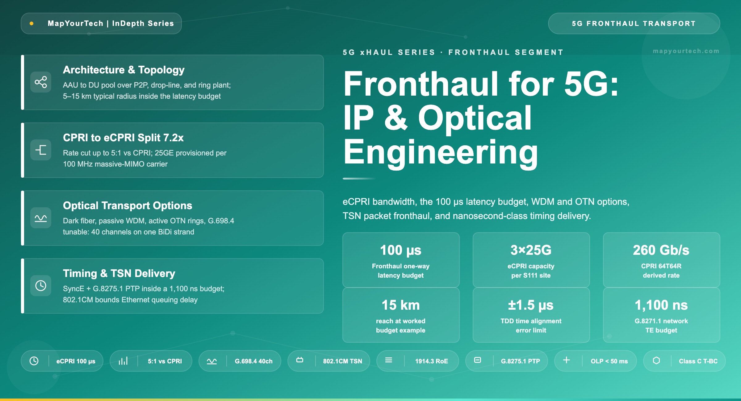
Fronthaul is the transport segment between the radio unit (RU, deployed as an active antenna unit, AAU) and the distributed unit (DU), and it is the only part of the 5G network where transport equipment carries radio-layer payload under radio-layer deadlines. A single S111 site with three AAUs presents 3 × 25 Gb/s of eCPRI interface capacity from the day the radio powers on, per operator planning estimates published in industry white papers, and every bit of it must arrive within a 100 µs one-way budget set by the hybrid automatic repeat request (HARQ) timing of the air interface. No other segment combines constant line-rate bandwidth, a microsecond-class latency bound, and a ±1.5 µs absolute time-alignment requirement in one link.

Those three constraints are why fronthaul gets its own engineering discipline rather than a corner of the backhaul design. This article covers the segment end to end: the architecture between AAU and DU pool, the requirement set that any candidate transport must satisfy, the bandwidth mathematics of CPRI and eCPRI, the four optical transport options and where each wins, packet fronthaul over time-sensitive Ethernet, synchronization delivery, and a product capability checklist usable in an RFP. The segment's position inside the full three-segment xHaul model is covered in the companion overview of 5G transport network architecture; this article goes deep on the RU–DU link alone.

2. Fronthaul Architecture

2.1 From C-RAN to the Disaggregated RU–DU Link

The fronthaul concept predates 5G. 4G centralized RAN (C-RAN) pulled baseband units out of cell sites into pooled hotel locations and connected them to remote radio units over CPRI, trading transport cost for pooling gain and simpler site engineering. 5G kept the pooling economics but moved the split point: the DU absorbs the real-time protocol layers (Radio Link Control, Medium Access Control, high physical layer) while the AAU keeps the low physical layer, beamforming, and the RF chain. The result is the O-RAN split 7.2x interface carried over eCPRI, replacing the raw I/Q sample stream of CPRI with frequency-domain data whose rate scales with traffic and spatial layers rather than antenna count.

The physical architecture has three fixed roles. AAUs sit on towers, rooftops, and street poles, each presenting one or more 10/25GE eCPRI ports on SFP28 optics. The DU pool sits in a central-office or aggregation-site equipment room, typically 5–15 km away, hosting baseband processing for tens of radios. Between them sits the fronthaul transport plant: the fiber, filters, and (in active designs) the WDM or OTN equipment this article evaluates in Section 5. How the DU pool then connects onward through the metro is the subject of the companion OTN architectures that support 5G.

2.2 Topology Families

Three topology families cover deployed fronthaul. Point-to-point runs a dedicated path per AAU: the simplest and lowest-latency form, used wherever feeder fiber is plentiful. Drop-line (chain) topologies run a single fiber past several sites, dropping wavelengths at each: a fit for road and rail corridors. Ring topologies share two feeder strands among many sites and add protection switching: the choice for dense urban plant where fiber is the scarce resource and survivability is mandatory. Industry deployment guidance frames the selection through concentration scenarios: moderate concentration favors direct fiber, heavy point-to-point concentration favors passive or tunable WDM, and heavy ring concentration favors active WDM/OTN with optical-layer protection.

3. Transport Requirements

Five requirement classes define fronthaul, and a candidate transport must satisfy all five simultaneously. The numbers below come from the eCPRI specification, 3GPP timing requirements, the ITU-T G.8271.1 budgeting framework, and operator planning estimates published in industry white papers.

3.1 The Requirement Set

Bandwidth is provisioned, not grown: each AAU presents 10 or 25 Gb/s of eCPRI interface from power-on, so an S111 site loads the transport with 3 × 25 Gb/s on day one. Latency is bounded at 100 µs one-way for the high-priority eCPRI user plane, a figure derived from HARQ round-trip timing; exceed it and the radio scheduler stalls. Synchronization must deliver ±1.5 µs of time alignment error at the air interface, decomposed into a 1,100 ns transport budget under G.8271.1. Availability follows the radio layer: baseband processing tolerates roughly 50 ms of interruption before sessions drop, so protected fronthaul must switch inside that bound. Fiber economics close the set: dense urban feeder cables rarely offer a strand per AAU port, so wavelength multiplexing or single-fiber bidirectional working is frequently mandatory rather than optional.

3.2 What the Requirements Exclude

The requirement set excludes more technologies than it admits. Conventional carrier Ethernet with statistical queuing fails the latency and delay-variation bounds unless the IEEE 802.1CM profile constrains it (Section 6). Deep packet buffers, useful everywhere else in the network, are a liability here because buffering is delay. Layer-3 routing inside the fronthaul adds lookup latency and timing-plane complexity with no compensating benefit on a link whose endpoints never change. The engineering posture is subtraction: every element between AAU and DU must justify its microseconds.

4. Bandwidth Engineering: CPRI to eCPRI

4.1 Why CPRI Does Not Scale to Massive MIMO

CPRI transports time-domain I/Q samples per antenna port at constant rate, with line rates defined up to 24.33 Gb/s (rate option 10) and no forward error correction, a deliberate omission to avoid coding latency. Its rate is set by the antenna count and sampling rate alone:

RCPRI = Nant × fs × Nbits × 2 × Ccw × Cline

Where:
  Nant   = antenna-carrier streams
  fs     = sampling rate (122.88 MHz for 100 MHz NR)
  Nbits  = bits per I or Q sample (typ. 15)
  2      = I and Q components
  Ccw    = control-word factor (16/15)
  Cline  = line coding (66/64 or 10/8)

Practical Example — 100 MHz, 64 ports, 15-bit, 64B/66B:
  R = 64 × 122.88M × 15 × 2 × 16/15 × 66/64 ≈ 260 Gb/s
  (≈ 315 Gb/s with 8B/10B coding — derived approximation
   under these stated assumptions)

260 Gb/s for one 64T64R carrier is the number that ended CPRI's role in 5G mid-band: it exceeds the highest CPRI rate option by an order of magnitude and is constant whether the cell serves one user or one thousand. CPRI persists in the network wherever 4G radios persist, carried natively over a wavelength or encapsulated into Ethernet via IEEE 1914.3 Radio over Ethernet.

4.2 The eCPRI Rate and the Reach Budget

eCPRI at split 7.2x moves beamforming into the RU, so the transported stream scales with spatial layers instead of antenna ports; O-RAN Alliance material puts the reduction at up to 5:1 against CPRI for the same carrier. The practical outcome is the provisioning rule operators use: one 25GE eCPRI port per 100 MHz massive-MIMO carrier, 10GE for smaller configurations. The rate is partially traffic-dependent, which is what makes statistical multiplexing in packet fronthaul possible at all.

Reach follows from the latency budget by subtraction. Light in G.652 fiber accrues 5 µs/km of group delay, so the distance envelope is:

Lmax = ( Tbudget − Tequipment − Tqueuing ) / 5 µs/km

Practical Example — maximum fronthaul reach:
  Budget 100 µs, DU processing margin 20 µs,
  switching/queuing 5 µs:
  Lmax = (100 − 20 − 5) / 5 = 15 km

Every active element spends the same currency: an active WDM node at ~1 µs costs 0.2 km of radius, a TSN switch hop with bounded queuing costs more. Transparent transport (dark fiber, passive filters) spends nothing, which is the root of its appeal on long feeders. The chart below shows the derived trade for a packet fronthaul as switch hops accumulate.

Figure 2: Per-AAU fronthaul rate, CPRI (derived from the rate formula above) versus provisioned eCPRI interface rate. The gap is the split-7.2x dividend.

5. Optical Transport Options

5.1 The Four Options

Dark fiber assigns each AAU port its own strand pair, or a single bidirectional strand with BiDi optics. It adds zero latency and zero equipment, and it exhausts feeder cables fastest: a 36-AAU DU pool needs 36–72 strands. Industry deployment guidance reserves it for moderate-concentration plant where feeder count at least equals AAU count.

Passive CWDM/DWDM compresses 6–48 flows onto one pair using colored optics in the AAU and DU plus athermal multiplexer/demultiplexer filters in the field. Filter delay is nanoseconds and nothing in the path needs power, but the link carries no optical-layer OAM, sparing becomes a per-wavelength inventory problem, and a failed filter port stays dark until a truck roll. The wavelength mechanics are covered in the MapYourTech explainer on what DWDM is and how it works.

Active WDM/OTN terminates the gray AAU interface and maps it into a managed wavelength; OTN-based systems use ODUk containers with 25 Gb/s tributary slots and reduced multiplexing layers keeping device latency near 1 µs. In exchange for that microsecond, the operator gets per-channel performance monitoring, alarms, optical line protection (OLP) and ODUk subnetwork connection protection (SNCP) inside 50 ms, aggregation for large AAU counts, and ring topologies that conserve feeder fiber. Hardened full-outdoor variants mount on towers and poles for sites without equipment rooms. Industry deployment guidance recommends active DWDM as the clear choice for heavily concentrated ring scenarios.

ITU-T G.698.4 (formerly G.metro) standardizes a tunable-laser, port-agnostic WDM access system: head-end equipment at the DU office and tail-end devices at the AAU auto-tune to assigned wavelengths on a grid supporting up to 40 channels over single-fiber bidirectional transmission. Tunability collapses colored sparing to one part number, the embedded message channel gives passive-style plant a management view, and BiDi working halves fiber consumption while symmetrizing the path for timing (Section 7).

6. Packet Fronthaul: Ethernet, TSN, and RoE

eCPRI's packet framing puts fronthaul onto Ethernet, and Ethernet brings statistical multiplexing: multiple RUs share switched capacity, and the partially traffic-dependent split-7.2x rate makes the sharing pay. The price is that switches queue, and queuing is exactly what the 100 µs budget cannot absorb unbounded. IEEE 802.1CM, the time-sensitive networking (TSN) profile for fronthaul, bounds it: Profile A uses strict priority for the eCPRI user plane, and Profile B adds frame preemption (IEEE 802.3br / 802.1Qbu) so a high-priority radio frame can interrupt a low-priority frame already on the wire, cutting worst-case interference delay to a fragment time.

Tblock = Lframe × 8 / Rline

Practical Example — blocking delay on a 25GE fronthaul port (derived):
  1,500 B standard frame : 1500 × 8 / 25×109 = 0.48 µs
  9,000 B jumbo frame    : 2.88 µs
  128 B preempt fragment : ≈ 41 ns

The arithmetic is the argument for Profile B: one jumbo frame already on the wire costs 2.88 µs of the 100 µs budget at every congested hop, while preemption caps the same event near 41 ns (derived for a 128-byte fragment). Multiply by hop count and the difference decides whether a multi-switch packet fronthaul closes its budget at all.

IEEE 1914.3 Radio over Ethernet (RoE) completes the converged picture by defining structure-aware and structure-agnostic mappings that encapsulate legacy CPRI flows into Ethernet frames. A 4G CPRI radio and a 5G eCPRI radio can then ride one packet fronthaul, one fiber plant, and one timing distribution, which is the deployment reality for any operator running both generations from shared sites.

The product consequence: a fronthaul-class Ethernet switch is judged on its bounded worst-case latency under the 802.1CM class targets, its preemption support, and its timing-plane behavior (Section 7), not on its buffer depth. Deep buffers, the selling point of data-center switching, are disqualifying here.

7. Synchronization Delivery

TDD radios transmit and receive on a shared raster, and the 3GPP bound is ±1.5 µs of time alignment error at the air interface. The transport network delivers that time because per-site GNSS fails on cost, urban-canyon visibility, and jamming resilience. The deployed mechanism pairs Synchronous Ethernet (SyncE) for physical-layer frequency with Precision Time Protocol (PTP, IEEE 1588) under the ITU-T G.8275.1 telecom profile for phase and time; the profile mandates full timing support, with every node a boundary clock that terminates and regenerates PTP, because each non-aware hop adds unmodeled delay variation the budget cannot absorb. The division of labor between frequency and phase is unpacked in the MapYourTech article on timing versus synchronisation in telecommunication networks.

The G.8271.1 framework allocates 1,100 ns of network time error from the primary reference time clock to the RU input. Fiber asymmetry is the field-dominant consumer: time offset equals half the forward/reverse delay difference, so a 10 m strand-length mismatch costs roughly 25 ns. This is why G.698.4's single-fiber bidirectional working is a timing feature as much as a fiber-economy feature, and why DWDM systems carry PTP over the optical supervisory channel with each node as a boundary clock, the approach detailed in OTN synchronization methods for 5G networks.

TEnetwork = TEPRTC + Σ cTEBC,i + TEasym + TEdynamic  ≤  1,100 ns

  TEasym = ( dforward − dreverse ) / 2

Practical Example — fiber asymmetry:
  10 m strand mismatch → Δd ≈ 50 ns → TEasym ≈ 25 ns

Holdover closes the design: on PTP path loss the slave free-runs on SyncE-disciplined oscillators while the timing plane recovers, with oscillator quality chosen for the required window. Redundant grandmasters and GNSS backup at aggregation sites (not every cell site) complete the protection picture; the scenario trade-offs are worked through in the MapYourTech synchronization methods decision tree.

8. Product Capabilities Checklist

The requirement set of Section 3 converts directly into procurement language. The capabilities below separate fronthaul-class equipment from general metro transport in an RFP; values marked typical vary by product class and should be confirmed against vendor specifications.

9. Deployment Scenarios and Design Rules

Three scenarios from industry deployment guidance cover most builds. Moderate concentration (suburban, fiber-rich): direct fiber or BiDi gray optics, point-to-point, no active equipment, reach limited only by the 15 km class budget. Heavy point-to-point concentration (urban, fiber-lean): passive DWDM or G.698.4 tunable systems compress 36+ flows onto one or two strands; G.698.4 wins where sparing logistics and timing symmetry matter. Heavy ring concentration (dense urban, shared feeder rings): active WDM/OTN with OLP, accepting ~1 µs per node for sub-50 ms survivability and full telemetry; the protection mechanics sit inside the broader decision space mapped in the MapYourTech deep dive on network protection in optical network architecture.

Four design rules then govern every scenario. Spend the latency budget on glass, not silicon: prefer transparent elements and count every active hop against the reach formula. Keep paths symmetric for timing: bidirectional working or matched strand lengths, recorded at acceptance. Protect at the layer that switches fastest: optical-layer OLP on rings, with ODUk SNCP where electrical-layer granularity is needed. Power and footprint discipline: street cabinets and tower enclosures impose hard limits, and per-bit energy comparisons between an active ring and a passive build with deeper DU pooling follow the pJ/bit framework in the MapYourTech analysis of energy efficiency in optical networks.

Figure 3: Remaining fronthaul reach versus active node count, derived from the Section 4.2 model (100 µs budget, 20 µs DU margin, 5 µs queuing, 1 µs per active node). Illustrative derived values; actual margins vary by vendor mode.

10. Automation and Operations

11. Evolution and Outlook

Fronthaul interface rates track radio bandwidth: 25GE eCPRI is the present default, with 50GE positioned for wider millimeter-wave carriers as those bands mature. On the optical layer, higher-channel-count tunable systems and pluggable-form-factor tail ends continue the G.698.4 direction of pushing the WDM function into the radio itself. On the packet layer, tighter 802.1CM class targets and wider frame-preemption support keep statistical fronthaul viable as per-cell rates climb.

The architectural pull is toward fewer, larger DU pools: every consolidation step raises AAU counts per feeder and pushes more plant from the moderate scenario into the heavy ones, which favors tunable and active WDM over time. Synchronization tightens in parallel, as inter-site coordination features in 5G-Advanced press relative-time requirements toward the hundreds-of-nanoseconds class and keep full-timing-support PTP non-negotiable on this segment.

Glossary

• AAU: Active Antenna Unit; the RU integrated with the antenna array and RF chain.
• CPRI / eCPRI: Common Public Radio Interface and its packet-based successor for fronthaul transport.
• DU: Distributed Unit; real-time baseband processing pooled at a central site.
• G.698.4: ITU-T tunable-laser, port-agnostic WDM access system used for fronthaul, formerly G.metro.
• HARQ: Hybrid Automatic Repeat Request; the air-interface retransmission process that sets the fronthaul latency budget.
• ODUk SNCP: Optical Data Unit subnetwork connection protection; electrical-layer 1+1 protection in OTN.
• OLP: Optical Line Protection; optical-layer fiber-route switching.
• Option 7.2x: The O-RAN intra-PHY functional split carried by eCPRI fronthaul.
• PTP / SyncE: Precision Time Protocol (phase/time) and Synchronous Ethernet (frequency) distribution.
• RoE: Radio over Ethernet (IEEE 1914.3); CPRI encapsulation into Ethernet frames.
• TAE: Time Alignment Error; the ±1.5 µs air-interface bound for TDD.
• TSN / 802.1CM: Time-Sensitive Networking profile bounding delay and loss for fronthaul over switched Ethernet.