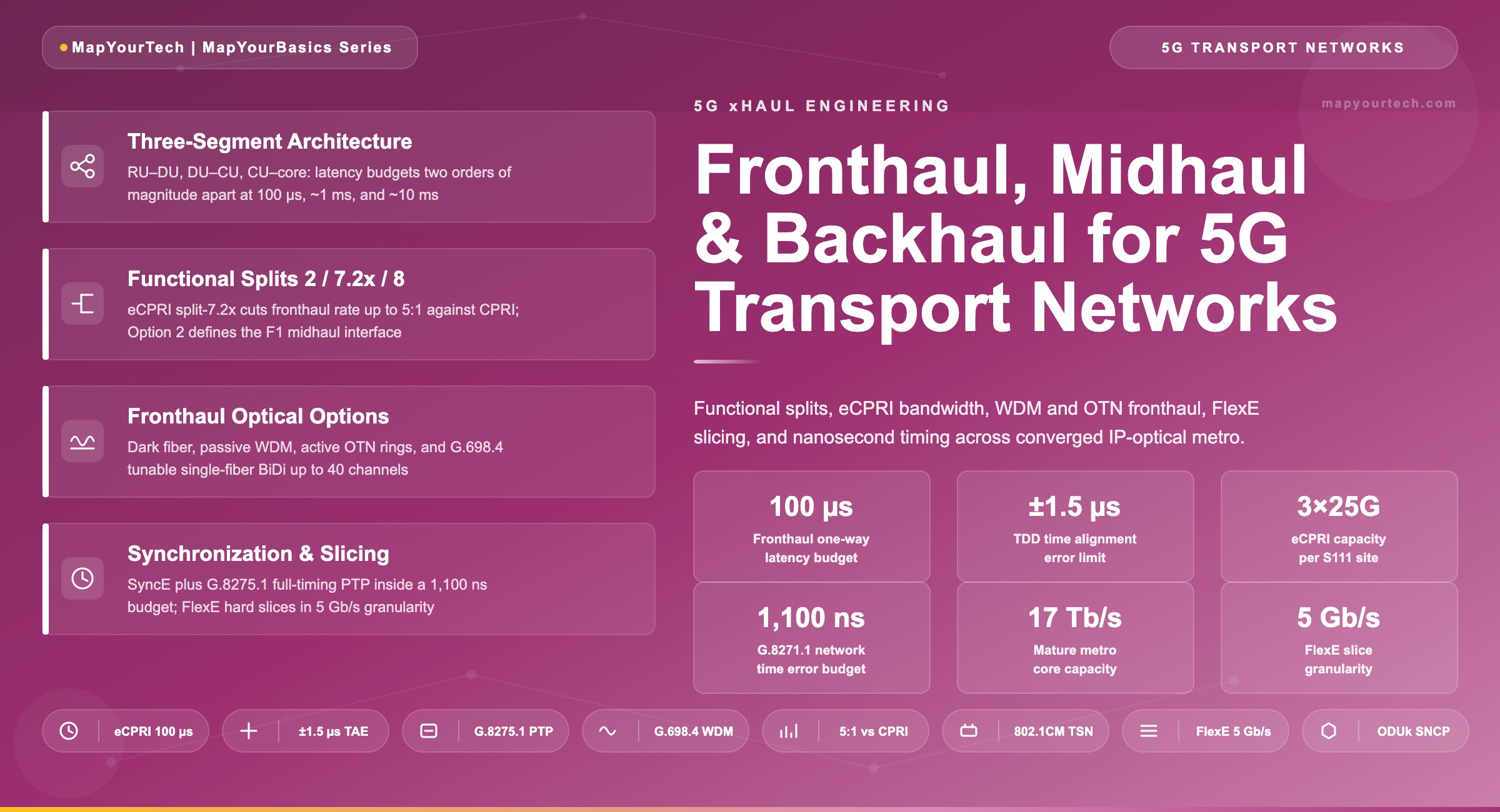
Fronthaul, Midhaul and Backhaul for 5G: Supporting IP and Optical Networks
How the three segments of 5G transport are engineered: functional splits, eCPRI bandwidth, latency budgets, WDM and OTN fronthaul, IP-optical convergence, and nanosecond-class synchronization.
1. Introduction
A 5G base station with 100 MHz of sub-6 GHz spectrum demands roughly 3 × 25 Gb/s of fronthaul capacity; operator planning estimates published in industry white papers put this at more than ten times the transport requirement of an equivalent LTE site. That single number explains why 5G forced a redesign of the access transport network rather than a simple upgrade. The radio access network (RAN) was disaggregated into three functional elements (the radio unit, the distributed unit, and the centralized unit), and each pair of elements created a transport segment with its own bandwidth, latency, distance, and synchronization profile. Those three segments are fronthaul, midhaul, and backhaul, collectively called xHaul.
Fronthaul carries time-critical radio samples with a one-way latency budget of 100 µs, set by the hybrid automatic repeat request (HARQ) timing of the air interface and codified in the eCPRI specification. Backhaul carries ordinary IP packets with budgets measured in milliseconds. Midhaul sits between them, carrying the F1 interface between distributed and centralized units. No single transport technology serves all three economically, which is why working networks combine dark fiber, passive and active wavelength-division multiplexing (WDM), packet-enhanced optical transport network (OTN) equipment, and IP routing with segment routing and Flexible Ethernet (FlexE) — each placed where its cost and performance profile fits.
This reference covers the full engineering chain: the architectural model and the 3GPP functional splits that define it, the bandwidth mathematics of Common Public Radio Interface (CPRI) and enhanced CPRI (eCPRI), latency budget calculations, the four fronthaul optical transport options and when each wins, the converged IP-optical design of midhaul and backhaul, the synchronization architecture that keeps time-division duplex (TDD) radios inside ±1.5 µs, and the dimensioning method for a metro network carrying thousands of sites. The material targets engineers who design, deploy, or operate mobile transport; the foundations are built in place so a reader new to xHaul can follow without a separate primer, and readers wanting the structural basics first can start with this overview of 5G transport network architecture.
2. The Three-Segment Architecture
2.1 From BBU and RRU to RU, DU and CU
4G networks split the base station into two boxes: a baseband unit (BBU) doing all digital processing and a remote radio unit (RRU) at the antenna. The link between them was the original fronthaul, carrying CPRI; the link from the BBU toward the core was backhaul. 5G split the BBU itself. The non-real-time protocol layers, Packet Data Convergence Protocol (PDCP) and Radio Resource Control (RRC), moved into a centralized unit (CU) that can serve many sites from a regional location. Radio Link Control (RLC), Medium Access Control (MAC), and the upper physical layer kept their real-time deadlines and became the distributed unit (DU). The RRU absorbed the lower physical layer and the antenna array to become the active antenna unit (AAU), referred to as the radio unit (RU) in O-RAN terminology.
Three elements create three links. Fronthaul connects the RU to the DU; midhaul connects the DU to the CU over the 3GPP F1 interface; backhaul connects the CU to the 5G core over the NG interface. When an operator collocates the CU and DU in one gNB, the integrated deployment preferred for ultra-reliable low-latency communication (URLLC) services because it removes one latency stage, the midhaul segment disappears and the network reverts to a two-segment structure. When the operator collocates the DU with the RU at the cell site (distributed RAN), the fronthaul segment shrinks to an intra-site cable and only midhaul and backhaul traverse the metro. The segment count is therefore a deployment decision, not a fixed property of 5G; the OTN architectures that support 5G span centralized RAN (C-RAN), distributed RAN (D-RAN), and hybrid placements of the same three functions.
2.2 Traffic Characteristics
North-south traffic dominates every segment. Operator measurements reported in industry white papers put east-west traffic (the inter-site coordination flows on the eX2/Xn interface carrying inter-site carrier aggregation and coordinated multipoint data) at roughly 10–20% of the S1/NG traffic volume, and that traffic flows only between geographically adjacent cells, never full-mesh. The transport consequence is direct: the access and aggregation layers can be engineered as aggregation trees with simplified IP forwarding rather than full mesh fabrics, while flexible any-to-any connectivity is reserved for the metro core where the cloudified core network and multi-access edge computing (MEC) sites interconnect.
Takeaway: Fronthaul, midhaul, and backhaul are defined by the RAN functional split, not by geography. RU–DU traffic is constant-rate, time-critical radio data with a 100 µs budget; DU–CU and CU–core traffic is statistical IP traffic with millisecond budgets. Collocating CU with DU removes midhaul entirely, so segment count is a deployment choice that the transport design must accommodate.
3. Functional Splits and Interface Protocols
3.1 The Split Options That Survived
3GPP TR 38.801 catalogued eight candidate split points through the radio protocol stack, but commercial deployment converged on three. Option 2 splits between PDCP and RLC and defines the CU/DU boundary: the F1 midhaul interface. Option 7.2x, specified by the O-RAN Alliance fronthaul working group, splits inside the physical layer between the high-PHY (channel coding, modulation mapping) and the low-PHY (beamforming, FFT/iFFT, cyclic prefix); it is the dominant fronthaul split for open RAN deployments. Option 8 splits between the low-PHY and the RF chain, transporting raw time-domain I/Q samples — the classic CPRI split inherited from 4G C-RAN.
The split point determines everything downstream. A lower split (Option 8) centralizes maximum processing and enables the tightest inter-cell coordination, but its bandwidth scales with the number of antenna elements and is traffic-independent: the link runs at full rate even when no user is attached. A higher split (Option 7.2x) keeps beamforming in the RU, so the fronthaul rate scales with spatial layers rather than antenna ports (O-RAN Alliance material puts the reduction at up to 5:1 against CPRI for the same carrier), and the rate becomes partially traffic-dependent, which unlocks statistical multiplexing in packet fronthaul. Option 2 carries close to user throughput plus protocol overhead, which is why midhaul dimensioning looks like ordinary IP capacity planning.
3.2 CPRI, eCPRI and Radio over Ethernet
CPRI is a constant-bit-rate, synchronous serial protocol with line rates defined up to 24.33 Gb/s (rate option 10), 8B/10B or 64B/66B coded, with no forward error correction — a deliberate omission to avoid coding latency. It assumes a transparent, deterministic pipe: dark fiber or a WDM wavelength. eCPRI, published by the CPRI Cooperation, repackages the split-7 payload into Ethernet or UDP/IP frames; the eCPRI specification states the 100 µs one-way latency requirement for its high-priority user-plane traffic class. Because eCPRI is packet-based, multiple RUs can share a switched Ethernet fronthaul, but the switches must then bound delay and delay variation, the role of the IEEE 802.1CM time-sensitive networking (TSN) profile for fronthaul. IEEE 1914.3 Radio over Ethernet (RoE) complements both by defining structure-aware and structure-agnostic mappings that encapsulate legacy CPRI flows into Ethernet frames, letting 4G CPRI and 5G eCPRI ride one converged packet fronthaul.
Takeaway: Option 7.2x with eCPRI is the deployment default because it cuts fronthaul bandwidth by up to 5:1 versus CPRI (O-RAN figure), makes the rate scale with spatial layers instead of antenna ports, and moves fronthaul onto Ethernet where 802.1CM TSN and statistical multiplexing apply. CPRI remains in the network wherever 4G radios persist, carried natively over WDM or encapsulated via IEEE 1914.3 RoE.
4. Bandwidth and Latency Engineering
4.1 The CPRI Rate Formula
CPRI bandwidth is deterministic arithmetic, which makes it the right place to see why Option 8 collapses under massive MIMO. The line rate is the product of antenna-carrier count, sample rate, sample width, and protocol overheads:
RCPRI = Nant × fs × Nbits × 2 × Ccw × Cline

Where:
  Nant   = number of antenna-carrier streams
  fs     = sampling rate (Hz); 122.88 MHz for a 100 MHz NR carrier
  Nbits  = bits per I or Q sample (typically 15)
  2      = I and Q components per sample
  Ccw    = control-word overhead = 16/15
  Cline  = line coding overhead = 66/64 (or 10/8 for 8B/10B rates)
A worked case shows the scaling problem. For a 100 MHz carrier (fs = 122.88 MHz), 64 antenna ports, 15-bit I/Q samples, and 64B/66B coding, the formula gives 64 × 122.88 × 106 × 30 × (16/15) × (66/64) ≈ 260 Gb/s, and approximately 315 Gb/s with 8B/10B coding — a derived approximation under these stated assumptions, and an order of magnitude beyond any pluggable gray optic an operator would place on a tower. The same radio under split 7.2x, where the fronthaul carries frequency-domain data per spatial layer rather than per antenna port, fits in the 25 Gb/s class for typical 8–16 layer configurations. That ratio, not any single standard clause, is the engineering reason eCPRI displaced CPRI for 5G massive MIMO.
4.2 The Fronthaul Latency Budget
The 100 µs eCPRI one-way budget converts directly into a reach limit because light in standard single-mode fiber propagates at roughly 5 µs per kilometer. The budget must also fund every active element in the path:
Tbudget ≥ Tfiber + Tequipment + Tqueuing

  Tfiber = L × 5 µs/km     (group delay in G.652 fiber, n ≈ 1.468)

Practical Example — maximum fronthaul reach:
  Tbudget    = 100 µs (eCPRI one-way, high-priority plane)
  Tequipment = 20 µs  (WDM mux/demux, two TSN switch hops, RU/DU PHY)
  Tqueuing   = 5 µs   (engineered worst-case under 802.1CM)
  Lmax = (100 − 20 − 5) / 5 = 15 km
This calculation explains the near-universal engineering rule that fronthaul stays within 10–20 km of the DU. Every switch hop, every active WDM transponder, and every queuing stage subtracts kilometers from the radius, which is why transparent transport (dark fiber or passive WDM with zero electrical processing) buys the longest reach, and why ring fronthaul topologies that accumulate per-node delay are engineered with strict hop counts. Midhaul and backhaul live under far looser constraints: 3GPP TR 38.913 sets the end-to-end user-plane targets these segments must fit inside: 4 ms for enhanced mobile broadband (eMBB) and 0.5 ms for URLLC between the terminal and the CU. These targets translate to midhaul reaches of tens of kilometers and backhaul reaches of 100–200 km in typical metro builds.
| Indicator | Latency | Source | Transport consequence |
|---|---|---|---|
| Fronthaul one-way (RU–DU) | 100 µs | eCPRI specification | 10–20 km reach, transparent or TSN-bounded transport |
| Terminal to CU, eMBB | 4 ms | 3GPP TR 38.913 | Midhaul within metro access/aggregation |
| Terminal to CU, URLLC | 0.5 ms | 3GPP TR 38.913 | Integrated CU/DU preferred; midhaul removed |
| Vehicle-to-everything (eV2X) | 3–10 ms | 3GPP TR 38.913 | MEC placement at aggregation layer |
| TDD air-interface time alignment | ±1.5 µs | 3GPP TDD requirement | Full-timing-support PTP through transport (Section 7) |
4.3 Bandwidth per Segment
Operator planning estimates published in industry white papers for a typical S111 site (one sector set, three AAUs) put fronthaul at 3 × 25 Gb/s from day one (the eCPRI interface rate is provisioned with the radio, not grown with traffic), while midhaul and backhaul start near 5 Gb/s peak / 3 Gb/s average per site with early 100 MHz spectrum and grow toward roughly 20 Gb/s peak / 9.6 Gb/s average as 800 MHz-class millimeter-wave spectrum matures. The asymmetry is the central dimensioning fact of xHaul: fronthaul is wide and flat, midhaul and backhaul are narrower and statistical.
Aggregation multiplies these per-site figures into core-layer requirements. The same operator estimates model a large metro with 12,000 5G sites and a 6:1 statistical convergence ratio reaching more than 6 Tb/s of core-layer capacity at the initial stage and about 17 Tb/s at maturity — the numbers that pushed 25G/50G interfaces into the access layer and 100G-and-above coherent wavelengths into the metro core. Section 8 works the dimensioning method in full.
Takeaway: Fronthaul reach is a subtraction problem: 100 µs minus equipment and queuing delay, divided by 5 µs/km, lands at 10–20 km. Fronthaul bandwidth is provisioned with the radio at 3 × 25 Gb/s per site regardless of load; midhaul/backhaul bandwidth follows user traffic from ~5 Gb/s peak early to ~20 Gb/s peak at maturity per operator planning estimates, and aggregates under a 4:1 to 6:1 convergence ratio.
5. Fronthaul Optical Transport Options
5.1 Direct Dark Fiber
Direct fiber is the lowest-latency, zero-equipment option: each AAU port gets its own fiber pair (or a single bidirectional strand) to the DU. Its failure mode is fiber exhaustion. A site with three AAUs consumes three or six strands; a centralized DU pool serving 30+ AAUs in a heavy-concentration scenario consumes the entire feeder cable, and dense urban duct space rarely supports that. Industry deployment guidance therefore reserves direct fiber for moderate-concentration scenarios where the feeder count at the central office is at least equal to the AAU count, and treats it as a transitional state everywhere else.
5.2 Passive WDM
Passive coarse or dense WDM compresses 6–48 fronthaul flows onto one fiber pair using colored optics in the AAU and DU plus athermal multiplexer/demultiplexer filters in the field — no powered equipment between the endpoints, hence no added latency beyond the filters' nanoseconds and no powered cabinet to lease. The trade-offs are operational: colored pluggables turn sparing into a per-wavelength inventory problem, a failed filter port is dark until a truck roll, and the link carries no optical-layer OAM, so fault isolation depends on the radios at each end. The wavelength mechanics behind these systems are covered in the MapYourTech explainer on what DWDM is and how it works.
5.3 Active WDM/OTN
Active fronthaul equipment terminates the gray AAU interface, maps it into a managed wavelength (for OTN-based systems, an ODUk container with 25 Gb/s tributary slots and reduced multiplexing layers keeping device latency near 1 µs) and provides what passive systems cannot: performance monitoring, alarm reporting, optical-layer protection (OLP) and electrical-layer ODUk subnetwork connection protection (SNCP), aggregation for large AAU counts, and ring topologies that conserve feeder fiber. Industry deployment guidance recommends active DWDM as the clear winner for heavily concentrated ring scenarios, where its protection switching and fiber economy outweigh its higher cost and the small latency it adds. Hardened full-outdoor variants mount on towers and poles for sites without equipment rooms.
5.4 The ITU-T G.698.4 Approach
ITU-T G.698.4 (formerly G.metro) standardizes a port-agnostic, tunable-laser WDM access system aimed squarely at fronthaul economics. Head-end equipment in the DU office and tail-end devices at the AAU (small boxes or enhanced pluggable modules inside the AAU) auto-tune to their assigned wavelength on a grid supporting up to 40 channels, over single-fiber bidirectional transmission. Tunability collapses the colored-optics sparing problem to one part number, the embedded messaging channel gives the passive-style plant a management view, and bidirectional working on one strand both halves fiber consumption and symmetrizes the path for timing (Section 7). Transparent transmission keeps latency and jitter at the physical-layer minimum, and the architecture supports point-to-point, drop-line, and ring builds with optical add/drop.
| Criterion | Direct fiber | Passive WDM | Active WDM/OTN | G.698.4 tunable |
|---|---|---|---|---|
| Fiber consumption | Highest (1–2 per AAU port) | Low (1 pair per site/ring) | Lowest (ring sharing) | Low (single-fiber BiDi) |
| Added latency | None | ~ns (filters only) | ~1 µs class per node | ~ns (transparent) |
| OAM and monitoring | None | None | Full (PM, alarms) | Embedded channel |
| Protection | None (re-route at RAN) | None | OLP, ODUk SNCP | Optical-layer options |
| Sparing model | Gray optics | Per-wavelength colored | Managed transponders | One tunable part |
| Best fit | Fiber-rich, moderate concentration | Moderate concentration, P2P | Heavily concentrated rings | P2P, drop-line, fiber-lean metros |
Practical Example — choosing between passive and active WDM: A DU pool serves 36 AAUs across a 14 km feeder ring with four splice points and two feeder strands available. Direct fiber is out (36 strands needed, 2 available). Passive DWDM fits the channel count but offers no protection on a ring whose whole point is survivability, and a single feeder cut would drop all 36 radios with no switching. Active DWDM with OLP restores the ring in under 50 ms at the optical layer and reports per-channel power telemetry to the NMS; the roughly 1 µs per-node latency cost subtracts only 0.2 km from the reach budget computed in Section 4.2. The ring scenario decides for active — exactly the recommendation in industry deployment guidance.
Takeaway: Fronthaul transport selection is a fiber-count and topology decision before it is a technology preference. Fiber-rich point-to-point plant favors direct fiber or passive WDM; fiber-lean or ring plant favors active WDM/OTN for its protection and OAM; G.698.4 tunable systems remove the colored-sparing penalty of passive WDM while keeping transparent latency, at up to 40 channels on a single bidirectional strand.
6. Midhaul and Backhaul: IP-Optical Convergence
6.1 Why These Segments Need IP
Backhaul carries two connection families: CU-to-core (the NG interface) and CU-to-neighbor-CU (the eX2/Xn interface for inter-site coordination). Static point-to-point circuits cannot follow CU cloudification: once a DU can re-home across two or more CU pools for redundancy and load sharing, the midhaul must resolve destinations dynamically, which means IP addressing and forwarding. The traffic matrix stays simple (north-south dominant, east-west only between neighbors), so the access and aggregation layers need simplified routing rather than a full internet-grade control plane, but they need routing nonetheless. The integrated CU/DU deployments used for URLLC push the same IP requirement down into what would otherwise be fronthaul-only territory.
6.2 Packet-Enhanced OTN and IP RAN
Two converged architectures dominate deployments. The first pairs packet-enhanced OTN in the access/aggregation layers with an IP RAN core: OTN devices gain MPLS-TP-based forwarding plus OSPF, IS-IS, BGP, and segment routing, exchange routes with the IP RAN via BGP, and carry IP/MPLS-TP over ODUk channels so that latency-critical flows ride one-hop optical paths while the electrical layer handles aggregation. The second runs an end-to-end IP RAN over a DWDM line system, increasingly with coherent pluggables directly in router ports — the routed optical networking model, whose coherent-versus-direct-detect selection boundaries determine where a 400G ZR-class pluggable replaces a transponder shelf. The interface ladder is consistent across both: 25GE and 50GE in access, 100GE in aggregation, N × 100GE or 400GE coherent wavelengths in the metro core. The container mechanics of ODUk mapping and multiplexing are covered in the complete guide to optical transport networks.
6.3 Network Slicing: FlexE Hard Isolation and Soft QoS
5G defines three service classes: eMBB, URLLC, and massive machine-type communication (mMTC). Network slicing gives each class its own virtual network with independent resources. The transport layer implements slicing at two hardnesses. FlexE shims a calendar-based time-division layer between Ethernet MAC and PHY, carving a 100GE PHY into channels in 5 Gb/s granularity whose traffic cannot contend with each other: hard isolation, suitable for a URLLC slice that must never see an eMBB burst in its queue. ODUk channels provide the same hard isolation at the OTN layer with one-hop pass-through at intermediate nodes. Soft slicing (VPN instances, hierarchical QoS, segment routing traffic engineering with flex-algo) shares capacity statistically and suits eMBB/mMTC separation where isolation is administrative rather than physical. Production designs layer them: FlexE or ODUk for the URLLC slice, SR-based soft slices for the rest.
6.4 Protection and Restoration
xHaul availability targets are inherited from the radio layer: baseband processing tolerates roughly 50 ms of transport interruption before calls and sessions drop, so every segment is engineered to sub-50 ms recovery. Fronthaul rings use optical-layer OLP or ODUk SNCP; IP midhaul and backhaul use segment routing with topology-independent loop-free alternate (TI-LFA) fast reroute, which pre-computes backup paths for link, node, and shared-risk failures. The full protection-architecture decision space, from SNCP through TI-LFA to circuit-style SR for timing-critical flows, is mapped in the MapYourTech deep dive on network protection in optical network architecture.
Takeaway: Midhaul and backhaul are IP networks riding optical capacity, not circuits. Packet-enhanced OTN brings MPLS-TP, IGP/BGP, and SR into the transport layer and exchanges routes with the IP RAN; FlexE and ODUk supply hard slice isolation in 5 Gb/s granularity for URLLC while SR-based soft slices carry eMBB and mMTC; TI-LFA and SNCP keep every segment under the 50 ms recovery bound the radio layer demands.
7. Synchronization Architecture
7.1 The Requirement
5G NR is deployed predominantly as TDD, and TDD only works if every cell in an interference domain switches between transmit and receive inside a common time raster: the 3GPP requirement is ±1.5 µs of time alignment error at the air interface, the same bound as 4G TDD. Coordination features tighten it further: the 5G air-interface frame is 1 ms against 4G's 10 ms, shrinking the margin available to inter-site carrier aggregation and coordinated multipoint, whose relative-time requirements fall into the hundreds-of-nanoseconds class. The transport network is the delivery vehicle for this time, because equipping every street-level site with a GNSS receiver fails on cost, on urban-canyon visibility, and on jamming resilience.
7.2 SyncE plus PTP with Full Timing Support
The deployed architecture pairs two mechanisms. Synchronous Ethernet (SyncE) distributes frequency through the physical layer by locking every Ethernet line rate to a primary reference, giving parts-per-billion stability that survives packet load. Precision Time Protocol (PTP, IEEE 1588) distributes phase and time-of-day through timestamped messages; the ITU-T G.8275.1 telecom profile mandates full timing support, with every node in the path a boundary clock that terminates and regenerates PTP, because each non-aware hop adds unmodeled delay variation that the ±1.5 µs budget cannot absorb. The division of labor between the two mechanisms, and why frequency alone is insufficient for TDD, is unpacked in the MapYourTech article on timing versus synchronisation in telecommunication networks.
Time error budgets are allocated per hop. The end-to-end network limit from the primary reference time clock (PRTC) to the RU input is 1,100 ns in the G.8271.1 budgeting framework, decomposed across the PRTC itself (±100 ns), each boundary clock's constant time error contribution, and link asymmetries. Two physical-layer details dominate field results: fiber asymmetry between transmit and receive strands converts directly into time offset at half the delay difference, which is why single-fiber bidirectional working (native in G.698.4 fronthaul) is also a timing feature; and on DWDM systems, carrying PTP over the optical supervisory channel gives a low-jitter, symmetric path with each node acting as a boundary clock, the approach detailed in OTN synchronization methods for 5G networks.
TEnetwork = TEPRTC + Σ cTEBC,i + TEasym + TEdynamic  ≤  1,100 ns

  TEasym = ( dforward − dreverse ) / 2

Practical Example — fiber asymmetry:
  A 10 m length difference between Tx and Rx strands
  Δd = 10 m × 5 ns/m = 50 ns  →  TE asym = 25 ns
  Forty such uncompensated joints exhaust the entire 1,100 ns budget.
7.3 Holdover and Resilience
Timing fails differently from traffic: a PTP path loss does not drop the radio immediately, it starts a clock drift race. Designs therefore specify holdover, where the slave free-runs on SyncE-disciplined oscillators while the timing plane recovers, with oscillator quality chosen for the required holdover window, from hours on temperature-compensated parts to days on better references. Redundant grandmasters, GNSS at aggregation sites as backup rather than at every cell site, and automatic source selection complete the design; the trade-offs among these protection scenarios are worked through in the MapYourTech synchronization methods decision tree.
Takeaway: TDD makes synchronization a transport deliverable: ±1.5 µs at the air interface, budgeted as 1,100 ns through the network under G.8271.1. The architecture is SyncE for frequency plus G.8275.1 full-timing-support PTP for phase, with every transport node a boundary clock; fiber asymmetry at 25 ns per 10 m of strand mismatch is the silent budget killer, and single-fiber bidirectional working neutralizes it.
8. Design and Dimensioning
8.1 The Capacity Model
Metro xHaul dimensioning runs bottom-up: per-site rates, multiplied by site count, divided by the statistical convergence ratio at each aggregation stage. Fronthaul does not converge (eCPRI interfaces are provisioned at line rate), so convergence applies from the midhaul up, where traffic is statistical. A defensible model uses 4:1 to 6:1 between access and core depending on busy-hour correlation across the served area.
Ccore = ( Nsites × Rsite,avg ) / Kconv

Where:
  Nsites    = number of 5G sites in the metro
  Rsite,avg = average per-site mid/backhaul rate (Gb/s)
  Kconv     = statistical convergence ratio (4–6 typical)

Practical Example — large metro (operator planning estimates):
  Nsites = 12,000   Kconv = 6
  Early (R = 3 Gb/s avg):   C = 12,000 × 3 / 6  = 6 Tb/s
  Mature (R = 9.6 Gb/s):    C = 12,000 × 9.6 / 6 ≈ 17–19 Tb/s
8.2 Topology, Latency and Power Trade-offs
Topology selection trades fiber economy against latency accumulation. A ring shares fiber and protects itself, but transmission delay accumulates node by node: an eight-node access ring with even modest per-node processing erodes a meaningful fraction of a midhaul latency budget, which is why industry guidance recommends migrating latency-critical layers from ring toward tree topologies, where only source-to-sink hops count. Device-level countermeasures move in the same direction: 25 Gb/s tributary slots instead of 5 Gb/s reduce multiplexing stages, buffer minimization targets device latency near 1 µs, and ODUk pass-through lets intermediate nodes forward optically-framed traffic without packet processing.
Power and footprint close the design loop. Every active fronthaul element sits in a constrained street cabinet or tower enclosure, and the metro aggregation sites absorb the multiplied port counts, so per-bit energy becomes a selection criterion alongside latency and cost; the pJ/bit accounting framework in the MapYourTech analysis of energy efficiency in optical networks applies directly to comparing an active fronthaul ring against a passive build plus deeper DU pooling.
8.3 Design Checklist
- Fix the RAN placement first: C-RAN, D-RAN, or hybrid determines which segments exist and at what reach.
- Run the latency subtraction (Section 4.2) per fronthaul path, including every planned switch hop and WDM element, before committing topology.
- Dimension fronthaul at interface line rate; dimension midhaul/backhaul on peak/average traffic with an explicit convergence ratio and a documented growth step to the mature-spectrum case.
- Allocate the 1,100 ns time-error budget per hop at design time; verify fiber asymmetry on every bidirectional-pair route.
- Choose hard-slice capacity (FlexE/ODUk) for URLLC commitments before soft-slice policy design.
- Engineer every segment to sub-50 ms recovery and verify the protection mechanism per layer (OLP/SNCP at optical, TI-LFA at IP).
Takeaway: Dimensioning is bottom-up arithmetic with one discontinuity: fronthaul never converges, everything above it does. A 12,000-site metro at a 6:1 ratio lands at 6 Tb/s of core capacity early and roughly 17 Tb/s at maturity per operator planning estimates — the numbers that set 25G/50G access, 100G aggregation, and coherent 100G+ core as the standard interface ladder.
9. Deployment, Validation and Troubleshooting
9.1 Bring-up Sequence
Field experience converges on a strict order: physical plant, then timing, then transport, then radio. Fiber characterization comes first: insertion loss, OTDR trace, and connector inspection per span, with bidirectional length matching recorded for timing-critical routes. Timing comes second because a radio brought up on bad time produces interference that masquerades as a dozen other faults: validate SyncE traceability, PTP grandmaster reachability, and measured time error at the RU handoff against the per-hop budget before any eCPRI flow starts. Transport validation then exercises the eCPRI/RoE path with traffic generation (throughput at line rate, frame loss, latency, and packet delay variation against the 802.1CM class targets), and only then does RAN integration begin.
9.2 Common Faults and Their Signatures
| Symptom | Likely root cause | Diagnostic approach | Resolution |
|---|---|---|---|
| TDD interference, dropped uplink across a cluster | Time error beyond ±1.5 µs (PTP path fault, asymmetry) | Measure TE at RU with a calibrated probe; walk boundary-clock chain | Repair PTP path; compensate or re-splice asymmetric strands |
| eCPRI frame loss under load, radio resets | Fronthaul congestion or TSN misconfiguration | PDV/loss test per 802.1CM class; check switch queue config | Apply frame preemption/priority; re-dimension links |
| Single AAU dark, others on same fiber fine | Failed colored optic or filter port (passive WDM) | Per-channel power at mux/demux; loopback at AAU | Replace pluggable; clean/replace filter port |
| Whole ring of radios lost | Feeder fiber cut without optical protection | OTDR from hub; check OLP switch state if equipped | Splice repair; add OLP/SNCP if absent |
| Midhaul latency spikes during failures | IGP reconvergence instead of fast reroute | Compare failover time against 50 ms target | Enable TI-LFA; pre-compute backup paths |
| One slice degrades when another bursts | Soft slicing where hard isolation was required | Per-slice counters under synthetic load | Move URLLC slice to FlexE/ODUk channel |
Practical Example — isolating a timing fault: A cluster of 12 TDD cells on one aggregation ring reports rising uplink block error rate every afternoon. Spectrum analysis shows cross-cell interference, not external ingress. A time-error probe at two RU handoffs measures +1.9 µs and +2.1 µs against GNSS reference, beyond the ±1.5 µs limit. Walking the boundary-clock chain finds one aggregation node whose PTP port fell back to a partial-timing profile after a software upgrade, adding unmodeled delay variation. Restoring G.8275.1 full timing support on that node returns measured TE to 240 ns and clears the interference. The afternoon pattern was load-correlated queueing delay through the non-aware hop — the signature that distinguishes a timing-plane fault from an RF one.
Takeaway: Bring up timing before traffic and verify it with measurement, not configuration review: most cluster-wide RF mysteries in TDD networks are transport time-error faults. Keep the fault tree layered: optical power and OTDR for physical, TE probes for timing, PDV/loss tests for packet fronthaul, failover timers for IP protection.
10. Technology Comparison and Selection
10.1 CPRI Versus eCPRI
| Attribute | CPRI (Option 8) | eCPRI (Option 7.2x) |
|---|---|---|
| Payload | Time-domain I/Q per antenna port | Frequency-domain data per spatial layer |
| Rate behavior | Constant, traffic-independent | Partially traffic-dependent; statistical multiplexing possible |
| Scaling driver | Antenna ports (breaks at massive MIMO) | Spatial layers (up to 5:1 reduction per O-RAN) |
| Framing | Synchronous serial, rates to 24.33 Gb/s | Ethernet/UDP-IP packets, any Ethernet rate |
| Transport assumption | Transparent pipe (fiber, WDM wavelength) | Switched Ethernet with 802.1CM TSN bounds |
| Timing delivery | Embedded in line code | SyncE + PTP through the packet network |
| Coordination ceiling | Maximum (full centralization) | High; beamforming stays in RU |
| 2026 role | Legacy 4G radios; RoE encapsulation for convergence | Default for 5G and open RAN fronthaul |
10.2 Selection Guidance by Scenario
Three deployment patterns cover most builds. A fiber-rich suburban operator with moderate DU concentration runs direct fiber or passive CWDM/DWDM fronthaul and an IP RAN midhaul/backhaul over leased or owned wavelengths: minimum equipment, minimum latency, acceptable because fiber is not the scarce resource. A dense urban operator with heavy DU pooling on ring plant runs active WDM/OTN or G.698.4 fronthaul for fiber economy and protection, packet-enhanced OTN aggregation with FlexE hard slices, and coherent DWDM in the core. A national operator converging fixed and mobile runs the OTN/WDM multi-service model, where 5G xHaul, residential broadband, and enterprise private lines share one transport with per-service ODUk or FlexE isolation — the unified-transport argument that operator white papers make on cost grounds: one network to power, one to operate, one to spare.
11. Where the Architecture Is Heading
Fronthaul rates step up next. 25 Gb/s eCPRI interfaces saturate as operators aggregate more spectrum per radio, and the component industry's answer is the same non-coherent toolkit that lifted fronthaul from 10G to 25G: PAM4 and discrete multi-tone DSP techniques that multiply rate over low-baud optics for sub-20 km reach, with 50 Gb/s-class fronthaul interfaces the published direction in operator technology white papers. In parallel, 50G PON developed under ITU-T's higher-speed PON family is positioned by several vendors as a shared-fiber small-cell fronthaul/backhaul option where dedicated WDM is uneconomic.
Midhaul and backhaul ride the coherent pluggable curve. The OIF 400ZR generation put DWDM interfaces directly into router ports for 80 km-class links, OpenZR+ extended modulation flexibility and reach for regional spans (the differences are detailed in the MapYourTech comparison of ZR versus ZR+ coherent optical standards), and the OIF 800ZR implementation agreement published in late 2024 brought general-availability 800G ZR/ZR+ coherent pluggables by 2025, doubling metro-core wavelength capacity in the same router faceplate. For the 17 Tb/s-class mature-metro core computed in Section 8, that progression is the difference between a wavelength-count problem and a routine upgrade.
Architecturally, 3GPP 5G-Advanced (Release 18 onward) deepens the coordination features (multi-TRP transmission, tighter positioning) that press synchronization toward the hundreds-of-nanoseconds class and keep full-timing-support PTP non-negotiable. SDN-based hierarchical controllers now span the optical and IP layers in production metros, computing latency-bounded paths and provisioning slices end to end; the open fronthaul management plane from the O-RAN Alliance gives the RU population the same programmability. The through-line of the roadmap is convergence: one packet-optical transport, sliced per service, timed from one reference, carrying everything from eCPRI to enterprise wavelengths.
12. Quick Reference
| Parameter | Fronthaul | Midhaul | Backhaul |
|---|---|---|---|
| Endpoints / interface | RU–DU, eCPRI / CPRI / RoE | DU–CU, F1 | CU–core, NG (N2/N3) |
| One-way latency class | 100 µs (eCPRI) | ~1 ms | ~10 ms |
| Typical reach | 10–20 km | 20–80 km | 80–200+ km |
| Per-site rate (S111) | 3 × 25 Gb/s provisioned | 5 Gb/s peak early, ~20 Gb/s mature | Same class as midhaul |
| Interface ladder | 10/25 GE gray or colored | 25/50/100 GE | N × 100 GE / 400 GE coherent |
| Transport options | Fiber, passive WDM, active WDM/OTN, G.698.4 | Packet OTN, IP RAN, FlexE | IP/MPLS + SR over DWDM/ROADM |
| Protection | OLP, ODUk SNCP | TI-LFA, SNCP | TI-LFA, restoration |
| Synchronization | SyncE + G.8275.1 full-timing-support PTP; ±1.5 µs at air interface; 1,100 ns network budget | ||
Essential Formulas
- CPRI rate: R = Nant × fs × 2 × Nbits × (16/15) × line-code overhead
- Fronthaul reach: Lmax = (100 µs − Tequipment − Tqueuing) / 5 µs/km
- Asymmetry time error: TE = (dfwd − drev) / 2 ≈ 25 ns per 10 m strand mismatch
- Core capacity: C = (Nsites × Ravg) / Kconv, with Kconv = 4–6
Glossary
- AAU: Active Antenna Unit; the RU integrated with the antenna array and RF chain.
- CPRI / eCPRI: Common Public Radio Interface and its packet-based successor for fronthaul transport.
- CU / DU / RU: Centralized, Distributed, and Radio Units of the disaggregated 5G RAN.
- F1 / NG: 3GPP interfaces carried by midhaul (DU–CU) and backhaul (CU–core) respectively.
- FlexE: Flexible Ethernet; calendar-based channelization of an Ethernet PHY in 5 Gb/s granularity for hard slice isolation.
- G.698.4: ITU-T tunable-laser, port-agnostic WDM access system used for fronthaul, formerly G.metro.
- HARQ: Hybrid Automatic Repeat Request; the air-interface retransmission process that sets the fronthaul latency budget.
- MEC: Multi-access Edge Computing; core functions placed at the metro aggregation layer.
- ODUk SNCP: Optical Data Unit subnetwork connection protection; electrical-layer 1+1 protection in OTN.
- OLP: Optical Line Protection; optical-layer fiber-route switching.
- Option 2 / 7.2x / 8: The surviving RAN functional splits: PDCP/RLC, intra-PHY (O-RAN), and PHY/RF.
- PTP / SyncE: Precision Time Protocol (phase/time) and Synchronous Ethernet (frequency) distribution.
- TI-LFA: Topology-Independent Loop-Free Alternate; segment-routing fast reroute with pre-computed backups.
- TSN / 802.1CM: Time-Sensitive Networking profile bounding delay and loss for fronthaul over switched Ethernet.
- URLLC / eMBB / mMTC: The three 5G service classes that drive slicing requirements.
References
- [1] 3GPP TR 38.913, Study on Scenarios and Requirements for Next Generation Access Technologies, 3GPP.
- [2] CPRI Cooperation, "eCPRI Interface Specification, Common Public Radio Interface."
- [3] O-RAN Alliance, "O-RAN Fronthaul Working Group Control, User and Synchronization Plane Specification."
- [4] ITU-T G.698.4, Multichannel bi-directional DWDM applications with port agnostic single-channel optical interfaces, ITU-T.
- [5] ITU-T G.8275.1, Precision time protocol telecom profile for phase/time synchronization with full timing support from the network, ITU-T.
- [6] IEEE 1914.3, Standard for Radio over Ethernet Encapsulations and Mappings, IEEE.
- [7] IEEE 802.1CM, Time-Sensitive Networking for Fronthaul, IEEE.
- [8] Sanjay Yadav, "Optical Network Communications: An Engineer's Perspective" — Bridge the Gap Between Theory and Practice in Optical Networking.
Related Articles on MapYourTech