
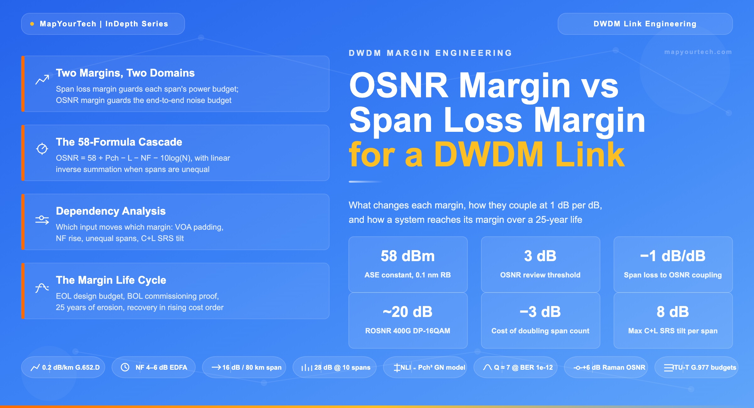
OSNR Margin vs Span Loss Margin in DWDM Links: What Changes Them and How a System Reaches Its Margin
Every DWDM link carries two independent margins: a power-domain span loss margin measured span by span, and a noise-domain OSNR margin measured end to end. This reference defines both, derives the formulas that govern them, catalogs every mechanism that consumes them over a 20 to 25 year design life, and traces the path a system follows from end-of-life budget allocation to commissioning measurement to margin exhaustion.
1. Introduction
A 16 dB span that measures 19 dB three years after commissioning has lost no end-to-end optical power at the receiver, because the downstream amplifier raised its gain to compensate. What the link lost is 3 dB of span loss margin on that span and roughly 0.4 to 3 dB of OSNR margin end to end, depending on how many spans share the route. The two losses are not the same quantity, they erode at different rates, and they fail the service through different mechanisms. Confusing them is the single most common error in DWDM link reviews.
Span loss margin lives in the power domain. It answers the question: how many additional decibels of attenuation can this individual span absorb before an amplifier runs out of gain range, a receiver falls below its input window, or the per-span noise contribution rises beyond what the design assumed. OSNR margin lives in the noise domain. It answers a different question: how far above the receiver's required OSNR does the delivered end-to-end OSNR sit, after every amplifier in the chain has added its amplified spontaneous emission (ASE) and the fiber has added its nonlinear interference.
The distinction matters because amplified links hide power problems. In an unamplified link, extra loss shows up directly as reduced receiver power, and the power budget margin is the only margin. In an amplified DWDM link, automatic gain control restores the power after every span, so received power stays flat while the noise floor quietly rises. The service does not fail when power drops; it fails when the pre-forward-error-correction (pre-FEC) bit error rate crosses the FEC limit, which is an OSNR-domain event. ITU-T G-series system design guidance states this directly: systems without line amplifiers are budgeted on received power, while multichannel systems with line amplifiers are budgeted on the OSNR needed to meet the required BER.
This article serves design engineers allocating margins for a new route, operations teams interpreting a shrinking Q margin on a live wavelength, and architects deciding whether a degraded span needs a fiber repair, a Raman upgrade, or a modulation downshift. Section 4 derives the governing equations with worked numbers. Section 5 catalogs every mechanism that consumes each margin, from fiber aging at roughly 0.003 dB/km over 25 years to a single contaminated connector that adds 2 dB overnight. Section 6 isolates the dependencies: which input moves which margin, by how much, in equal-span and unequal-span chains, and in C-band-only versus C+L operation. Section 7 traces the full life cycle: how an end-of-life budget becomes a beginning-of-life commissioning measurement and then erodes toward the FEC threshold.
2. Two Margins, Two Budget Domains
2.1 Span loss margin: the power-domain reserve
Span loss is the total attenuation between the output of one amplifier site and the input of the next: fiber attenuation plus every splice, connector, and patch panel in between. On ITU-T G.652.D fiber at 1550 nm, cabled attenuation runs 0.18 to 0.25 dB/km depending on fiber vintage and installation quality, so an 80 km span typically presents 16 to 20 dB of loss before connectors are counted. The relationship between insertion loss and return loss across connectors and splices sets the component-level contributions that stack into this total.
Span loss margin is the headroom between the actual measured span loss and the maximum span loss the design can tolerate. The tolerance ceiling comes from three constraints, and the binding one varies by link. First, the downstream amplifier has a maximum gain; once span loss exceeds it, the amplifier can no longer restore channel power. Second, the amplifier input power floor: below a minimum input, the amplifier output OSNR collapses because the ASE it generates is fixed while the signal it receives keeps shrinking. Third, on unamplified spans, the receiver sensitivity floor applies directly.
2.2 OSNR margin: the noise-domain reserve
OSNR is the ratio of per-channel signal power to ASE noise power in a 0.1 nm (approximately 12.5 GHz) reference bandwidth, measured on an optical spectrum analyzer. Every erbium-doped fiber amplifier (EDFA) in the chain adds ASE, so OSNR can only decrease as the signal propagates; no amplifier improves it. The mechanism behind this one-way accumulation, and why every span adds ASE in proportion to its amplifier's noise figure, is the physical foundation of the OSNR budget.
OSNR margin is the difference between the OSNR delivered to the receiver and the required OSNR (ROSNR) of the transceiver, after subtracting propagation penalties. ROSNR is the minimum OSNR at which the transceiver's FEC still corrects all errors, measured back-to-back by loading ASE until the post-FEC BER departs from zero. A coherent 400G channel running DP-16QAM at approximately 63 GBd needs roughly 20 to 21 dB of OSNR per vendor-published mode tables, while the same 400G carried as DP-QPSK at approximately 125 GBd survives at roughly 17 to 18 dB. The dependence of OSNR requirements on symbol rate and modulation format drives this spread: ASE power scales with signal bandwidth, and constellation density sets the SNR each symbol needs.
2.3 Why the system fails in the OSNR domain
Automatic gain-controlled amplifiers decouple received power from accumulated loss. When span loss rises, the line system raises gain and the receiver keeps seeing its target input power; the power-domain symptom disappears at the next amplifier. The noise-domain consequence does not disappear: higher gain at the same noise figure means proportionally more ASE, so the end-to-end OSNR drops by approximately 1 dB for every 1 dB of added loss on that span, per the standard amplified-link relation. The service degrades invisibly until the pre-FEC BER approaches the FEC limit, at which point post-FEC errors appear abruptly rather than gradually. This cliff behavior is why coherent systems are monitored on OSNR margin and Q margin rather than on received power.
Read the Full Analysis with Premium
The remaining 89% of this article — the design numbers, trade-offs and field guidance — is part of MapYourTech Premium, along with the full premium library, courses and professional tools.
You May Also Like

-
Free
-
September 4, 2026

-
Premium
-
September 4, 2026

-
Premium
-
September 4, 2026