
Nonlinearity Compensation Approaches and Their Cost
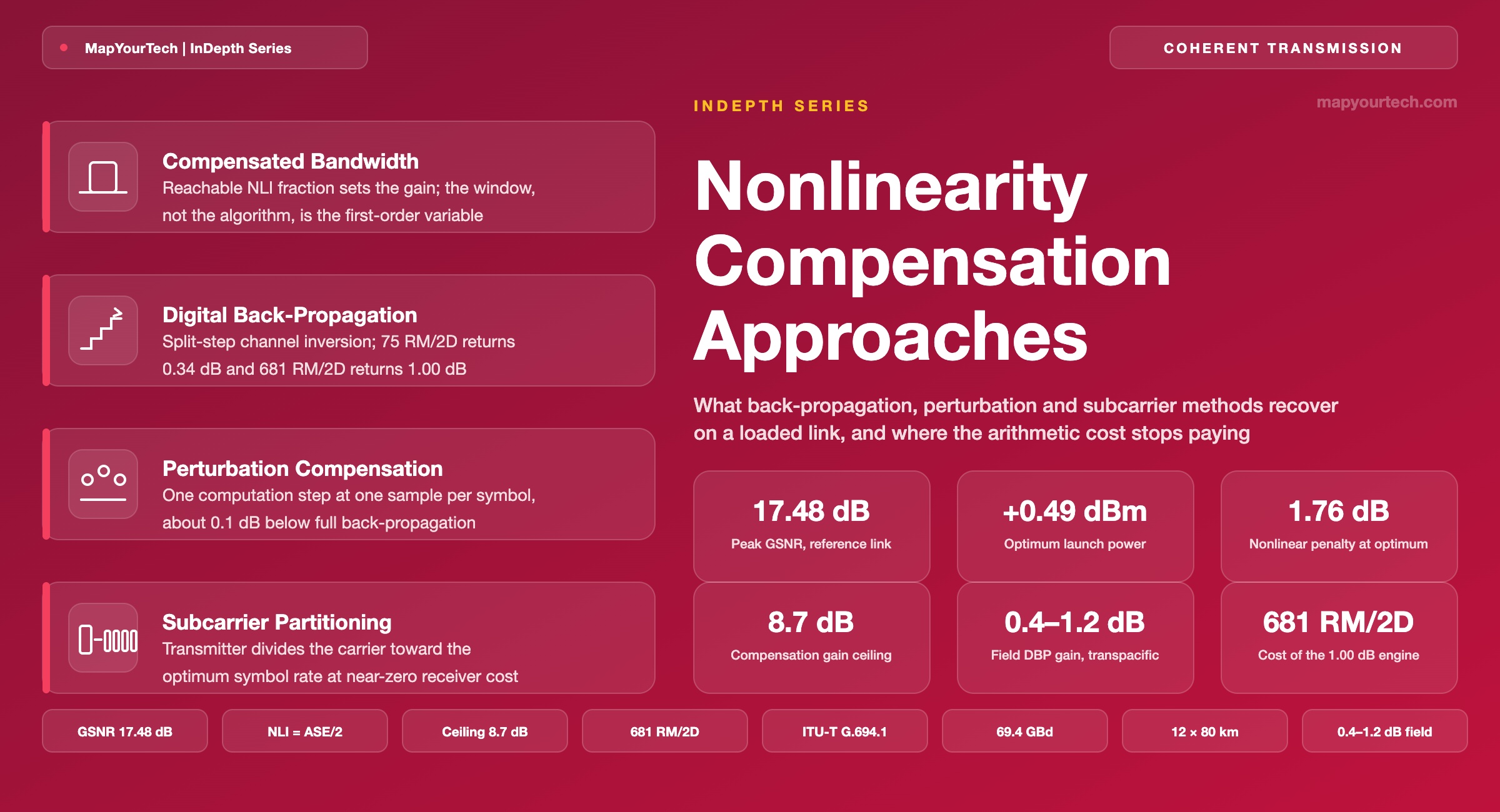
What digital back-propagation, perturbation methods and subcarrier partitioning each recover under fully loaded multi-channel conditions, what each costs in arithmetic and latency, and where the return stops justifying the processing.
The photons that close the budget are the photons that distort it.
What You Will Learn
- Define nonlinear interference and compensation gain from first principles, and state the 1.76 dB penalty that a link operating at its optimum launch power carries (Section 2).
- Quantify the fraction of nonlinear interference a compensator can reach from its observation window: 25% for one carrier, 68% for 1 THz, 90% for 4 THz on the reference link (Table 3).
- Derive the optimum launch power from the condition that nonlinear interference equals half the accumulated ASE power, and show why compensation gain appears as a power increase (Section 4.2).
- Compare the three compensator architectures by mechanism, observation window and failure boundary, using the block structures of Figures 4 to 6 (Section 5).
- Convert accumulated dispersion into an optimum subcarrier symbol rate, and apply the measured factor of three that places 69.4 GBd into four 17.35 GBd subcarriers (Section 6.1).
- Price a compensator in real multiplications per 2D symbol against the 32 required for linear equalization, and locate the point where the cost curve saturates (Table 4).
- Read a published compensation result correctly by checking channel count, occupied bandwidth, compensated bandwidth and both launch powers (Section 8.1).
- Select an approach for a given system class using route stability and receiver observation window as the first two tests (Figure 10, Table 6).
1. Introduction
A coherent transponder driven at 69.4 GBd over twelve amplified spans reaches its best performance at one launch power and degrades on either side of it. Below that power the amplified spontaneous emission (ASE) accumulated by the erbium-doped fiber amplifiers (EDFAs) dominates; above it the Kerr effect converts the extra photons into distortion faster than they add signal. The peak of that curve is where every long-haul link operates, and on the reference link used throughout this article it sits at +0.49 dBm per channel with a generalized signal-to-noise ratio (GSNR) of 17.48 dB. The nonlinear interference (NLI) present at that operating point costs exactly 1.76 dB against a link that had no Kerr effect at all.
That 1.76 dB is the prize. Nonlinearity compensation (NLC) exists to recover some part of it, and three families of technique have been developed to do so. Digital back-propagation (DBP) numerically reverses the propagation by solving the inverse nonlinear Schrodinger equation in the receiver. Perturbation methods expand the same equation to first order in the time domain and subtract a weighted sum of symbol triplets in a single computation step. Subcarrier partitioning changes the transmitted signal itself, dividing one high-baud carrier into several lower-baud subcarriers that generate less nonlinear interference in the first place. Each recovers a different fraction of the penalty, and each charges a different price in arithmetic, latency, and design rigidity.
The gap between what these techniques achieve in a laboratory and what they achieve on a loaded route is wide enough to have shaped a decade of product decisions. A single-channel experiment, where one carrier propagates alone or with a handful of neighbors, reports gains of several decibels. The same algorithm on a fully loaded 96-channel system returns a few tenths of a decibel. Nothing about the algorithm changed. What changed is the fraction of the nonlinear interference that the compensator can observe, and therefore the fraction it can reverse. On the reference link, a compensator that sees only the carrier of interest can reach 25% of the generated NLI; a compensator spanning 1 THz reaches 68%; the full 7.2 THz load is needed to reach all of it. Those three numbers, derived in Section 4, explain almost everything else in this article.
1.1 Scope and Boundary Conditions
This article covers digital nonlinearity compensation for coherent optical transmission over uncompensated single-mode fiber: digital back-propagation and its reduced-complexity variants, perturbation-based compensation, subcarrier partitioning, and the placement choice between transmitter and receiver. It quantifies what each recovers under multi-channel conditions, states the arithmetic cost in real multiplications per symbol, and identifies the operating boundaries beyond which each stops returning value. Optical phase conjugation appears where it bears on the comparison but is not developed in detail, because its cost sits in mid-link optical hardware rather than in transceiver arithmetic. Dispersion-managed links, which have different nonlinear statistics, are outside the scope.
The physical model throughout is the Gaussian Noise (GN) model and its enhanced form. That model treats nonlinear interference as additive Gaussian noise whose power spectral density depends on the transmitted signal spectrum, and it holds once chromatic dispersion has decorrelated the signal phases, which happens within the first two spans of an uncompensated coherent link. It weakens for low-baud carriers and for fiber with dispersion below about 4 ps/(nm·km). A fuller treatment of the model itself is available in the Gaussian Noise model reference, and the relationship between the modeled quantity and the measured one is set out in GOSNR versus OSNR.
1.2 Reference Link R1
Reference link R1 is a terrestrial long-haul route of the kind that carries most inter-city traffic: twelve 80 km spans of ITU-T G.652.D fiber with EDFA-only amplification, fully loaded on a 75 GHz flexible grid. Every calculation that follows uses it, so a gain quoted in Section 8 traces back to a launch power in Section 2.
| Parameter | Value | Evidence class |
|---|---|---|
| Span length | 80 km | design assumption |
| Span count | 12 (960 km total) | design assumption |
| Fiber type | ITU-T G.652.D | standard-specified |
| Attenuation coefficient | 0.20 dB/km | typical deployed value |
| Dispersion parameter | 16.7 ps/(nm·km) at 1550 nm | typical deployed value |
| Nonlinear coefficient | 1.3 W-1km-1 | typical deployed value |
| Amplifier noise figure | 5.0 dB | typical deployed value |
| Channel count and spacing | 96 carriers on a 75 GHz grid | design assumption |
| Occupied bandwidth | 7.2 THz | derived |
| Symbol rate per carrier | 69.4 GBd | design assumption |
| Accumulated dispersion | 16,032 ps/nm | derived |
| Optimum launch power | +0.49 dBm per channel | GN-model result |
| GSNR at the optimum | 17.48 dB | GN-model result |
| OSNR at the optimum (0.1 nm) | 24.92 dB | GN-model result |
The dispersion figure carries more weight than it appears to. At 16,032 ps/nm of accumulated dispersion, a 69.4 GBd symbol spreads across roughly 619 neighboring symbol periods by the time it reaches the receiver. That spreading is what randomizes the field and makes the Gaussian description valid, and it is also what makes any time-domain compensator expensive: the compensator has to hold and process that much memory. Fiber parameter selection and its effect on the nonlinear budget is developed further in fiber parameters and capacity.
1.3 Compensated Bandwidth as the First-Order Variable
Compensated bandwidth outranks algorithm sophistication in setting what a compensator returns: an ideal engine restricted to one carrier recovers less than a crude one spanning ten. The gain then completes only at a re-optimized launch power: a compensator enabled at the old operating point captures a bounded fixed-power part, and the unrealized remainder grows with the compensated fraction. And the cost curve saturates long before the gain curve does, which places the operating point that reaches a shipping application-specific integrated circuit (ASIC) far to the left of the best achievable performance. Those three statements organise the sections that follow.
Takeaway: Nonlinear interference costs a link operating at its optimum launch power 1.76 dB, and compensation recovers the fraction of that penalty which the compensator can observe. Compensated bandwidth is the first-order variable; algorithm sophistication is the second.
2. Nonlinear Interference and Compensation Gain Definitions
Nonlinear interference is the additive, noise-like distortion that the Kerr effect generates when the optical field of one or more carriers modulates the refractive index of the fiber, converting part of the transmitted power into components that fall inside the receiver bandwidth. It is measured as a power in watts, or as a power spectral density in watts per hertz, and it accumulates span by span alongside amplified spontaneous emission.
Two properties separate nonlinear interference from every other impairment in a coherent link. It is generated by the signal, so its power rises as the cube of the launch power while ASE stays fixed. And it is deterministic given knowledge of every field that produced it, which is what makes compensation conceivable at all. Amplified spontaneous emission is stochastic and no amount of processing removes it; nonlinear interference is a calculable function of symbols that the transmitter chose and the receiver can, in principle, recover.
Read the Full Analysis with Premium
The remaining 89% of this article — the design numbers, trade-offs and field guidance — is part of MapYourTech Premium, along with the full premium library, courses and professional tools.
You May Also Like

-
Free
-
September 4, 2026

-
Premium
-
September 4, 2026

-
Premium
-
September 4, 2026