Know Your Fiber First: Fiber Parameters and Capacity
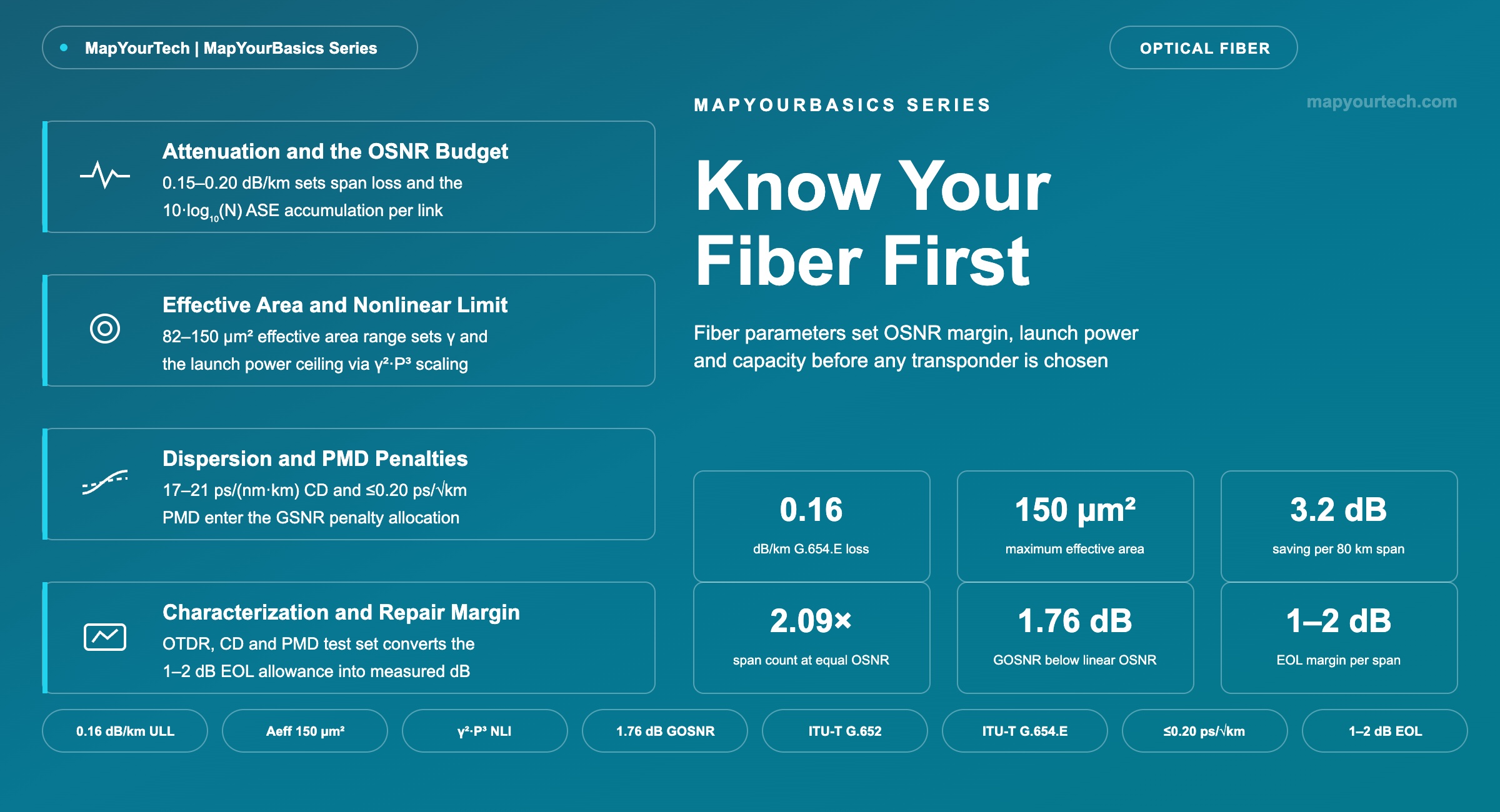
Attenuation, effective area, dispersion and PMD set the OSNR budget, the launch power optimum, the repair margin and the capacity ceiling of every wavelength before any transponder is chosen.
The true character of a fiber reveals itself under test.
1. Introduction
The fiber plant is the one layer of an optical transmission system that a software release cannot change and a hardware refresh rarely touches. Transponders turn over every three to five years, amplifiers and ROADMs every seven to ten, but the glass in the ground commonly serves for 25 years or more, and its four dominant parameters—attenuation, effective area, chromatic dispersion, and polarization mode dispersion (PMD)—fix the physical ceiling under which every later upgrade must operate. A planner who starts from channel counts and modulation formats without first measuring the fiber is solving the problem in the wrong order: the fiber decides the span loss, the span loss decides the Optical Signal-to-Noise Ratio (OSNR), the effective area decides how much launch power can push against that noise, and together they decide whether an 800 Gb/s wavelength closes the route or falls back to 400 Gb/s.
The point applies equally to new builds and to installed plant. On a new route, fiber selection is the single decision with the longest consequence horizon, because the difference between 0.20 dB/km and 0.16 dB/km compounds over every span for the life of the cable. On a brownfield route, the fiber is inherited, and the task becomes fiber characterization: measuring what the installed spans deliver so that capacity commitments rest on data rather than on nameplate assumptions. This overview maps each fiber parameter to its system consequence, compares the deployed fiber classes, sets out the characterization test set, and shows the margin arithmetic—OSNR margin, aging allowance, and repair margin—that converts measured fiber data into a defensible capacity plan.
2. Fiber Parameters and Their System Consequences
Four measurable fiber parameters determine the transmission potential of a route: the attenuation coefficient in dB/km, the effective area in µm², the chromatic dispersion coefficient in ps/(nm·km), and the PMD coefficient in ps/√km, supplemented by the splice and connector losses that sit on top of the bare glass. Figure 1 traces how each parameter feeds a physical mechanism—amplified spontaneous emission (ASE) accumulation, Kerr nonlinear interference (NLI), stimulated Raman scattering (SRS) power transfer, and linear penalty accumulation—and how each mechanism lands on a design outcome the planner must budget for.
2.1 Attenuation and the OSNR Budget
Attenuation is the parameter with the most direct line to capacity, because every amplified span converts fiber loss into ASE noise and OSNR accumulates span by span. Installed G.652.D plant typically measures 0.19–0.21 dB/km at 1550 nm including splices (measured field statistics reported in ITU-T G-series Supplement 39), commercial ultra-low-loss G.652 products are specified at 0.16 dB/km, G.654 classes reach 0.15–0.17 dB/km (commercial product specifications), and the laboratory record for silica-core fiber stands near 0.14 dB/km (measured laboratory record). For a route amplified with identical Erbium-Doped Fiber Amplifier (EDFA) spans, a widely used planning approximation ties these numbers to the received OSNR:
Multi-Span OSNR Planning Approximation
OSNRdB = 58 + Pch − Lspan − NF − 10·log10(N)
- Where:
- Pch = per-channel launch power in dBm (typical range −2 to +3 dBm for coherent channels)
- Lspan = loss of one span in dB, the product of the attenuation coefficient and span length plus splice losses (typical 14–22 dB for 80 km terrestrial spans)
- NF = amplifier noise figure in dB (typical 4.5–6 dB for a single-stage EDFA)
- N = number of identical amplified spans
- 58 = constant folding the ASE quantum noise floor into the 0.1 nm (12.5 GHz) reference bandwidth at 1550 nm (planning approximation)
Practical Example — span loss converted to OSNR on a ten-span route. Take ten 80 km spans at +1 dBm launch per channel and a 5 dB noise figure. On 0.20 dB/km fiber the per-span fiber loss is 0.20 dB/km × 80 km = 16 dB, and the formula gives OSNR = 58 + 1 − 16 − 5 − 10 = 28.0 dB. On 0.16 dB/km fiber the span loss falls to 12.8 dB and the OSNR rises to 31.2 dB—a fixed 3.2 dB advantage that holds at every span count (planning-model result). Because 3.2 dB equals 10·log10(2.09), the lower-loss fiber supports 2.09× the span count at any OSNR target, which Figure 2 shows as the 0.20 dB/km curve crossing an illustrative 28 dB threshold at 10 spans while the 0.16 dB/km curve crosses it at 21 spans.
Takeaway: Attenuation compounds linearly per kilometre but its OSNR consequence compounds over every span for the life of the route. A 0.04 dB/km difference is worth 3.2 dB per 80 km span, which is roughly the entire end-of-life margin allocation of many designs—the fiber class alone can double reach at a fixed required OSNR (planning-model result).
2.2 Effective Area and the Nonlinear Power Ceiling
If attenuation sets how fast the signal fades, effective area sets how hard it can be launched, because effective area governs every nonlinear impairment through the intensity of the guided mode. Silica’s nonlinear refractive index n2 is nearly constant across commercial fibers, so the nonlinear coefficient falls almost inversely with effective area:
Fiber Nonlinear Coefficient
γ = 2π·n2 / (λ·Aeff)
- Where:
- n2 = nonlinear refractive index of silica, approximately 2.6 × 10⁻²⁰ m²/W (measured material property)
- λ = signal wavelength, 1550 nm for C-band operation
- Aeff = effective area in µm² (82 µm² for G.652.D, 110–150 µm² for G.654 classes; commercial product specifications)
- γ = nonlinear coefficient in W−1·km−1 (typical 1.2–1.4 for G.652.D)
Practical Example — nonlinear coefficient and launch power headroom by fiber class. At 1550 nm with n2 = 2.6 × 10⁻²⁰ m²/W, an 82 µm² G.652.D fiber gives γ = 1.32 W−1·km−1, while a 125 µm² G.654.E fiber gives 0.87 W−1·km−1 (derived from the formula). Under the Gaussian Noise (GN) model, NLI power scales with γ²·P³, so holding NLI constant permits launch power to rise by two-thirds of the γ reduction in dB: 10·log10(1.32/0.87) = 1.8 dB of coefficient reduction buys about 1.2 dB of additional launch power (theoretical result). Combined with its lower loss, published planning guidance credits G.654.E with 2–3 dB of Generalized SNR (GSNR) advantage over G.652.D on new builds.
The GN model also fixes where the launch power optimum sits. Below the optimum, each added dB of launch power adds a dB of OSNR; above it, NLI grows three times faster than the signal and the generalized ratio falls. The two contributions combine as 1/GOSNR = 1/OSNRASE + 1/OSNRNLI in linear units, and at the optimum the achievable GOSNR equals two-thirds of the linear OSNR, a fixed 1.76 dB penalty (GN-model theoretical result). Larger effective area does not remove this penalty; it moves the whole curve upward by raising the power at which the optimum occurs. Effective area also enters stimulated Raman scattering in DWDM networks, where power transfers from shorter wavelengths to longer wavelengths and the shorter-wavelength channels are depleted: in wideband C+L band systems, published planning figures credit G.654.E with roughly 30–40% less SRS-induced tilt than G.652.D at equal total power, which reduces the pre-tilt and gain equalization the line system must apply.
Takeaway: Effective area is the second axis of fiber quality and the one that decides the launch power optimum. The γ²·P³ scaling means every 3 dB of nonlinear coefficient reduction converts to 2 dB of usable launch power at equal interference (theoretical result), and large-area fiber gains a second benefit in wideband systems through reduced SRS tilt.
2.3 Dispersion, PMD and Linear Penalty Allocation
Chromatic dispersion at 1550 nm runs near 17 ps/(nm·km) on G.652 and near 21 ps/(nm·km) on G.654 fiber (standard-specified typical values). For coherent transmission this accumulated dispersion is absorbed digitally in the receiver’s Digital Signal Processing (DSP), and moderate dispersion is beneficial because it decorrelates channels and suppresses four-wave mixing (FWM)—the mechanism behind the four-wave mixing problem that retired G.653 for DWDM use. The fibers that still demand caution are the low-dispersion legacy classes: G.653 spans place channels near the zero-dispersion wavelength where FWM products land directly on neighbouring channels, and mixed routes containing them constrain channel plans long after the transponders have gone coherent.
PMD behaves differently on new and old plant. Modern cabled fiber is specified at a PMD coefficient of at most 0.20 ps/√km (standard-specified, ITU-T G.652), and factory fiber commonly measures below 0.05 ps/√km (commercial product specifications), levels a coherent DSP equalizes without penalty. Cables installed before the mid-1990s, however, can measure several times the modern specification (measured field experience), and while coherent receivers track tens of picoseconds of differential group delay, high-PMD sections still raise outage probability at 130 GBd-class symbol rates and interact with polarization dependent loss (PDL), which remains an uncompensated penalty of typically 0.1–0.3 dB per concatenated component (typical planning values). In margin terms, CD, PMD and PDL enter modern planning tools as penalty entries subtracted from the path GSNR rather than as hard limits—small individually, but part of the budget the fiber decides.
Takeaway: Coherent DSP moved dispersion and PMD from hard limits to budget entries, but only for fiber that meets modern specifications. Legacy low-dispersion and high-PMD plant still constrains channel plans and symbol rates, which is why these parameters are measured, not assumed, before capacity is committed.
2.4 Raman Amplification Dependence on Fiber Parameters
Distributed Raman amplification turns the transmission fiber itself into the gain medium. A high-power pump, usually counter-propagating and placed about 100 nm below the signal band—near 1455 nm for C-band amplification, a 13.2 THz frequency offset—transfers power to the signal channels through stimulated Raman scattering (SRS) as it propagates back along the span. Because the span fiber is the amplifier, every parameter in this section reappears a second time as an amplifier parameter, and whether Raman amplification is worth deploying on a route is itself a fiber-parameter question. MapYourTech carries a foundational treatment of how a Raman amplifier works for readers arriving at this from the EDFA side.
On-Off Raman Gain Planning Form
Gon-off,dB ≈ 4.343·CR·Pp·Leff with CR = gR/Aeff and Leff = (1 − e−αpL)/αp
- Where:
- CR = Raman gain efficiency in W−1km−1 (typically 0.3–0.4 W−1km−1 for G.652 fiber with a depolarized counter-propagating pump)
- gR = Raman gain coefficient of the glass; about 2.8 × 10⁻¹⁴ m/W near 1500 nm for pure silica (standard-specified, ITU-T submarine-system guidance), raised by germanium doping
- Pp = pump power in W (typical 0.3–1 W per pump for terrestrial distributed Raman)
- αp = attenuation coefficient at the pump wavelength in km−1; around 0.25 dB/km for G.652 near 1455 nm, higher than the 1550 nm value (typical)
- Leff = effective interaction length in km; about 17 km for an 80 km G.652 span evaluated at the pump wavelength
Two dependences follow directly from the efficiency term. First, CR scales inversely with effective area, so the same large Aeff that lowers the nonlinear coefficient γ in section 2.2 also lowers the Raman gain each watt of pump delivers—the fiber chosen for its launch power headroom is the fiber that costs the most pump power to Raman-amplify. Second, gR depends on the glass composition: germanium doping raises it, so a pure-silica-core G.654 fiber starts from a lower coefficient than germanosilicate G.652 before the area scaling is applied (published gain-scaling measurements). Both effects push large-area ultra-low-loss routes toward higher pump powers, which brings connector power-handling and optical safety procedures into the span design.
The geometry of the gain matters as much as its magnitude. With a counter-propagating pump, the pump power—and therefore the gain—concentrates in the final Leff, roughly the last 17 km of the span nearest the receive end. A high-loss splice or a degraded connector inside that region subtracts almost directly from the achievable on-off gain, and a strong reflection there raises multipath interference through double Rayleigh scattering and can trigger the pump's automatic power reduction. The OTDR trace of the pump-side span end and the optical return loss (ORL) of its connectors are therefore Raman qualification items, measured under the same characterization discipline as section 4. The benefit that justifies this discipline is noise: because the signal receives gain before it falls to the span's noise floor, a distributed Raman stage reaches an effective noise figure near 0 dB or below, a result MapYourTech examines in its effective noise figure analysis of Raman amplification, and hybrid Raman-plus-EDFA spans use that headroom to extend reach on OSNR-limited routes.
Practical Example — pump power on G.652 versus G.654.E. Take an 80 km span with a 500 mW depolarized counter-propagating pump. On G.652 fiber with CR = 0.35 W−1km−1 and Leff ≈ 17.2 km at the pump wavelength, the planning form gives Gon-off = 4.343 × 0.35 × 0.5 × 17.2 ≈ 13.1 dB (planning arithmetic with typical values). Moving the same pump to a 125 µm² G.654.E fiber scales CR by 82/125 to about 0.23 W−1km−1 and the gain to about 8.6 dB; recovering 13.1 dB requires roughly 0.76 W, about 1.5 times the pump power, before the lower gR of a pure-silica core is counted. The route that gains the most from large effective area in launch power pays part of it back in Raman pump power.
Takeaway: The fiber decides not only how much amplification a span needs but how efficiently distributed Raman amplification can supply it: effective area and glass composition set the gain efficiency, pump-wavelength attenuation sets the interaction length, and splice and connector quality in the last roughly 17 km before a counter-propagating pump determines how much of the computed gain the span delivers.
3. Fiber Type Comparison and Selection Trade-offs
The deployed single-mode fiber classes differ most in the two parameters that matter most: attenuation and effective area. Table 1 compares the classes a planner encounters in terrestrial networks, with values drawn from commercial product specifications and standard-specified ranges.
| Parameter | G.652.D | G.652 Ultra-Low-Loss | G.655 (NZDSF) | G.654.E |
|---|---|---|---|---|
| Attenuation (dB/km) | 0.18–0.20 | 0.16–0.17 | 0.19–0.22 | 0.15–0.17 |
| Effective area (µm²) | ~82 | ~82 | 55–72 | 110–150 |
| Chromatic dispersion (ps/(nm·km)) | ~17 | ~17 | 2–8 | ~21 |
| Nonlinear coefficient γ (W−1·km−1) | 1.2–1.4 | 1.2–1.4 | 1.5–2.0 | 0.7–1.0 |
| Core composition | Ge-doped silica | Pure silica | Ge-doped silica | Pure silica |
| Primary deployment | Metro, regional, access | Long-haul upgrade builds | 1990s–2000s long-haul, legacy | New long-haul core routes |
The selection logic follows from Section 2. Where routes are short—metro rings and Data Center Interconnect (DCI) under roughly 200 km—the OSNR delivered by G.652.D already exceeds what high-order formats require, and the price premium of G.654.E buys margin the design cannot use. Where routes run long, the arithmetic reverses: field demonstrations have carried a real-time 1.6 Tb/s superchannel over 1600 km of G.654.E fiber and 12 wavelengths of 800 Gb/s over 1122 km (measured conference demonstrations), distances at which G.652.D would require regeneration or a rate step-down. G.655 serves coherent systems poorly: its smaller effective area raises γ above standard fiber, and the low dispersion that justified it in the 10 Gb/s era carries no benefit for a coherent receiver. Routes mixing fiber types add one further cost: the mode-field mismatch at a G.652-to-G.654.E joint contributes additional splice loss, typically around 0.1–0.2 dB per joint (typical field values), which mixed-fiber budgets must carry explicitly, and per-channel power targets differ by fiber class in mixed channel rate planning.
Practical Example — fiber selection on a 1000 km new build. A 13-span, 1040 km route at 80 km per span delivers an ASE-limited OSNR of 26.9 dB on 0.20 dB/km fiber and 30.1 dB on 0.16 dB/km fiber under the Section 2.1 assumptions (planning-model result). The 3.2 dB difference, plus roughly 1 dB of nonlinear headroom from the larger effective area, is the gap between operating 800 Gb/s wavelengths with usable margin and operating them at the edge of the format’s requirement. Over a 25-year cable life spanning perhaps five transponder generations, the fiber premium is paid once; the OSNR advantage is collected by every generation.
Takeaway: Fiber class selection is a one-time decision that repays or penalizes every transponder generation the cable will ever carry. G.652.D remains the correct answer for short reach; G.654.E earns its premium wherever span count and target rate push the OSNR and nonlinear budgets together (planning-model result).
4. Fiber Characterization and Margin Planning
Characterization converts an inherited fiber route from an assumption into a data set. It is performed after new construction, after a dark-fiber purchase or lease, and before any upgrade that raises symbol rate or channel count, because the parameters that decide feasibility—span loss, splice quality, dispersion, PMD—vary between the design record and the installed reality. Table 2 lists the standard test set and the typical acceptance thresholds applied to high-speed coherent routes.
| Test | Parameter Measured | Typical Acceptance Threshold | Consequence When Out of Specification |
|---|---|---|---|
| OTDR trace, both directions | Distributed attenuation, splice and connector events, reflectance | ≤0.1 dB per fusion splice; no unexplained point events (typical field thresholds) | High-loss splices consume span budget; reflective events degrade transmitter performance |
| Insertion loss (OLTS) | End-to-end span loss at operating wavelengths | ≤0.22 dB/km at 1550 nm including splices (typical acceptance threshold) | Span OSNR falls below the design value; amplifier gain and tilt settings drift from plan |
| Chromatic dispersion analysis | CD coefficient and slope across the band | Consistent with the declared fiber type curve | Reveals undeclared G.653 or mixed-type sections that constrain the channel plan |
| PMD analysis | Link differential group delay statistics | Coefficient ≤0.20 ps/√km (standard-specified for modern cabled fiber) | High-PMD sections raise outage probability at high symbol rates |
| Spectral attenuation profile | Loss versus wavelength, including the water peak region | Within the fiber class specification across intended bands | Blocks L-band or multiband expansion that the nameplate suggested was available |
Measured fiber data then feeds the margin stack. A coherent link closes when the path GSNR exceeds the transceiver’s required OSNR plus the allocated margins, and the fiber plant owns most of the entries: an aging and repair allowance of typically 1–2 dB per span covers connector degradation, splice aging and the accumulated cost of repairs over the service life (typical planning allocations), on top of the CD, PMD and PDL penalty entries of Section 2.3. Repair margin has concrete arithmetic behind it: each fiber cut repair inserts two fusion splices and a length of replacement cable, adding on the order of 0.1–0.5 dB per event depending on splice quality and inserted length (typical field values), and a route crossing exposed terrain accumulates these events for decades. The full allocation discipline—beginning-of-life versus end-of-life budgets and where each dB sits—is treated in BOL and EOL margin design, the measurement sequence at turn-up in the DWDM commissioning workflow, and the dependency chain from fiber parameters through GSNR to service margin in link engineering correlations.
Practical Example — upgrade decision on a legacy ten-span route. An operator plans 400 Gb/s wavelengths on a 15-year-old ten-span route with a design record claiming 0.22 dB/km. Characterization measures 0.24 dB/km average including aged splices, two splices at 0.4 dB each, and a PMD coefficient of 0.15 ps/√km. The extra 0.02 dB/km costs 1.6 dB of span loss over 80 km spans, and re-splicing the two events recovers 0.6 dB—the difference between launching the service with 2 dB of end-of-life margin and launching it with none (measured-and-computed example with typical field values). The characterization campaign costs days; discovering the shortfall after service commitment costs a regeneration site.
Takeaway: Margins are not abstractions layered on a design; they are dB quantities determined by the fiber plant. Characterization before commitment converts the aging, repair and penalty allowances from assumptions into measured quantities, and the cost of measuring is orders of magnitude below the cost of a missing dB found in service.
5. Standards Coverage and Industry Support
The fiber parameter framework rests on a compact set of ITU-T Recommendations. ITU-T G.650.1 and G.650.2 define the parameters themselves and their test methods, covering the linear deterministic attributes and the statistical and nonlinear attributes respectively. The fiber classes are specified in ITU-T G.652 (standard single-mode, current edition 2024), G.653 (dispersion-shifted, legacy), G.654 (cut-off shifted, current edition 2024, including the G.654.E subcategory for terrestrial coherent transmission), G.655 (non-zero dispersion-shifted), G.656 (wideband non-zero dispersion) and G.657 (bend-insensitive access fiber). ITU-T G-series Supplement 39, revised in 2025, carries the system design and engineering considerations that connect fiber attributes to link budgets, and ITU-T G.694.1 defines the flexible frequency grid the channels occupy.
Commercial support is broad and current. Sumitomo Electric specifies its PureAdvance G.654.E series at 0.16 dB/km or lower with 110 µm² and 125 µm² effective areas (vendor specifications), Corning lists ultra-low-loss G.652 and G.654 products in the same attenuation class (vendor specifications), and G.654.E has moved from trial to mainstream core-network practice: national operators in China deployed full G.654.E land trunk routes beginning in 2021, and industry analyses published in 2026 report the majority of new long-haul core routes specifying attenuation below 0.17 dB/km (published market reports). Interoperability at the system layer is unaffected by fiber class—coherent transceivers operate across all single-mode classes—but planning tools from the major line-system vendors model fiber type explicitly, because per-channel power optima, SRS tilt and NLI all shift with the fiber beneath them.
6. Fiber Technology Outlook
Silica fiber is approaching its material limits, and as of 2026 development is advancing on both sides of that limit. On the silica side, incremental attenuation and effective-area gains continue, and multiband transmission—super-C plus super-L systems approaching 12 THz of usable spectrum—extracts more capacity from the installed parameter set rather than changing it. Beyond silica, hollow-core fiber crossed a threshold: a double-nested antiresonant nodeless design published in Nature Photonics in 2025 measured 0.091 dB/km at 1550 nm, below the roughly 0.14 dB/km floor of the best silica fiber, with loss under 0.2 dB/km across a 66 THz window (measured, peer-reviewed result), and Microsoft has stated that on the order of 1200 km of hollow-core fiber already carries live cloud traffic (vendor statement). Because the guided mode travels in air, hollow-core also cuts one-way latency by roughly one-third and lowers the nonlinear coefficient by orders of magnitude, which would relocate the launch power optimum entirely.
None of this changes the discipline this article describes; it extends it. Whatever the fiber—installed G.652.D, new G.654.E, or an air-guided core—the parameter set of attenuation, effective area, dispersion and PMD remains the layer that sets the ceiling, and the operators who deploy each new transponder generation first will be the ones who measured their fiber before they committed its capacity.
Takeaway: The fiber parameter framework outlives any single fiber technology. Measure the four parameters, map them to OSNR, launch power and margin, and every future upgrade decision reduces to arithmetic on known quantities.
References
- ITU-T Recommendation G.652 — Characteristics of a single-mode optical fibre and cable, ITU-T Study Group 15.
- ITU-T Recommendation G.654 — Characteristics of a cut-off shifted single-mode optical fibre and cable, ITU-T Study Group 15.
- ITU-T G-series Supplement 39 — Optical system design and engineering considerations, ITU-T Study Group 15.
- ITU-T Recommendation G.650.1 — Definitions and test methods for linear, deterministic attributes of single-mode fibre and cable, ITU-T Study Group 15.
- Petrovich et al. — Broadband optical fibre with an attenuation lower than 0.1 decibel per kilometre, Nature Photonics.
- Sanjay Yadav, "Optical Network Communications: An Engineer's Perspective" — Bridge the Gap Between Theory and Practice in Optical Networking.
Related Articles on MapYourTech