
Ultralong-Haul Transmission in Submarine Optical Systems
A research-grade technical reference covering noise modeling, nonlinear physics, GSNR framework, and capacity design — with fully interactive formula calculators for design engineers.
“Noise accumulates, and nothing in a fiber ever removes it.”
Introduction
Submarine optical cable systems carry the majority of intercontinental data traffic, carrying the vast majority of all international data traffic across oceans. The engineering challenge — transmitting hundreds of terabits per second across transoceanic distances of 6,000 to 20,000 km using repeaters powered over a single high-voltage conductor — has no parallel in terrestrial networking. Every design decision carries irreversible financial and physical consequences, since deployed cable systems operate on the ocean floor for 25 years or more, far beyond the reach of ordinary maintenance.
The discipline of submarine optical transmission design is an optimization problem. Engineers must simultaneously balance optical signal-to-noise ratio (OSNR), fiber nonlinear effects, cable powering limits, dispersion management, and spectral efficiency — all under the constraint that repeaters cannot be accessed after deployment. This article provides a rigorous technical treatment of the physical models that govern system performance, the analytical frameworks used to predict and optimize capacity, and the transition from single-fiber optimization toward space division multiplexing (SDM) as the architecture of the current decade.
The treatment covers the entire signal impairment hierarchy: amplified spontaneous emission (ASE) noise from cascaded optical amplifiers, fiber Kerr nonlinearities modeled through the Gaussian Noise (GN) model, and the recently characterized guided acoustic-wave Brillouin scattering (GAWBS) effect. These three independent but interacting noise sources define the Generalized Signal-to-Noise Ratio (GSNR), which is the central figure of merit in modern open submarine cable characterization, standardized under ITU-T G.977.1.
Scope of This Article
This article addresses repeatered long-haul submarine systems operating in the C-band and C+L-band. Unrepeatered and direct-detection systems are outside the scope. All formula derivations reference established models from ITU-T recommendations and peer-reviewed optical communications literature. Every interactive calculator uses these exact formulas, allowing engineers to explore design trade-offs directly within the article.
Generalized Signal-to-Noise Ratio Definition and Component Terms
Generalized signal-to-noise ratio (GSNR) is the ratio of received per-channel signal power to the total power of every additive impairment the coherent receiver cannot distinguish from noise: amplifier ASE, Kerr nonlinear interference, and guided acoustic-wave Brillouin scattering. GSNR is dimensionless, quoted in decibels, and referenced to the symbol rate rather than to a fixed optical bandwidth.
Figure 1: Received channel power divided by the summed ASE, nonlinear-interference and GAWBS noise powers, with the reciprocal composition rule and the worked reference case beneath.
2.1 Distinctions From the Adjacent Quantities
Three quantities are routinely conflated, and each conflation changes the answer by more than a decibel. OSNR counts only amplifier ASE, measured in a fixed 0.1 nm reference bandwidth, and reports nothing about nonlinear distortion; a planning tool quoting 22 dB OSNR and a receiver reporting 19 dB SNR are measuring different things rather than disagreeing, as the analytical relationship between GOSNR and OSNR sets out. SNR at the receiver is referenced to the symbol rate and includes transponder implementation noise, so it sits below GSNR by the back-to-back penalty of the modem. GSNR sits between them: it is a property of the optical path alone, referenced to the symbol rate, and excludes transponder noise so that a wet plant can be specified independently of whoever terminates it.
Two further pairs matter. Reference bandwidth against symbol rate: OSNR is bandwidth-dependent and SNR is not, which is why the two only reconcile through an explicit conversion, treated at length in the OSNR fundamentals primer. Noise variance against noise power spectral density: the GN model produces a density that must be integrated over the channel bandwidth before it can enter the reciprocal sum above.
2.2 Units and Conversion Arithmetic
  1 / GSNR  =  Σi  1 / SNRi

  OSNRdB  =  SNRdB  +  10 · log10( Rs / 12.5 )
GSNR, SNRi — generalized and per-mechanism signal-to-noise ratios, linear units (not decibels)
Rs — symbol rate in GHz; typical submarine range 60–100 GBd
12.5 GHz — the 0.1 nm reference bandwidth at 1550 nm (standard-specified, ITU-T G.697)
The arithmetic runs one way only. Convert each contribution to linear units, sum the reciprocals, invert, then convert the result back to decibels. Summing decibel values directly is the most common error in this calculation and always overstates the penalty.
2.3 Worked Instantiation
Take the reference case this article returns to throughout: an 8,000 km route, 100 repeaters at 80 km spacing, 0.150 dB/km attenuation, 18 dBm total output power across 100 channels, 4.5 dB noise figure, and 125 µm² effective area. The three contributions evaluate to SNRASE = 25.5 dB (linear 356.5), SNRNL = 17.0 dB (linear 49.5), and SNRGAWBS = 21.7 dB (linear 149.2). Their reciprocals sum to 0.002805 + 0.020203 + 0.006702 = 0.029709, and the inverse of that is 33.7, or 15.3 dB of GSNR. Nonlinear interference contributes 68.0% of the total noise variance, GAWBS 22.6%, and ASE 9.4% — this case runs above the nonlinear threshold, and the Section 7 optimum moves the split back toward ASE.
Takeaway: GSNR is a reciprocal sum, so the smallest SNR term dominates the result and no amount of improvement in the other terms can recover it. Every design decision in the sections that follow — span length, launch power, effective area, fiber pair count — moves one of the three reciprocals, and the binding constraint is whichever one is largest.
System Architecture and Building Blocks
A repeatered submarine cable system consists of a small number of fundamental elements whose interaction governs all performance outcomes. Understanding each element — and precisely how it contributes to noise — is the necessary foundation before any formula can be applied meaningfully.
3.1 The Amplified Span
The fundamental building unit is an amplified span: a length of transmission fiber terminated at each end by an erbium-doped fiber amplifier (EDFA). Each repeater in a modern submarine cable houses multiple EDFAs — one per fiber pair direction — that compensate exactly for the span loss accumulated over the preceding fiber section. Span lengths in submarine systems typically range from 50 to 100 km, with the repeater spacing set at manufacture and fixed for the cable lifetime.
EDFAs amplify the signal through stimulated emission in the erbium-doped fiber, but they also generate amplified spontaneous emission (ASE) noise, which accumulates irreversibly with each repeater traversal. The noise figure (NF) of each EDFA — typically 4 to 6 dB in modern submarine repeaters — quantifies how efficiently signal power is added relative to noise power. A lower noise figure directly translates to a higher end-to-end OSNR for a given cable length and span configuration.
3.2 Fiber Types and Their Role
The transmission fiber used in submarine cables directly affects both the linear (ASE-dominated) and nonlinear noise budgets. Two fiber parameters govern system performance:
Effective area (Aeff): A larger effective area reduces the optical power density within the fiber core, proportionally reducing all Kerr nonlinear effects. Premium submarine fibers achieve effective areas of 125–150 µm², compared to 80–110 µm² for standard single-mode fiber. The nonlinear noise power scales approximately as 1/Aeff², so a fiber with 150 µm² effective area generates roughly 4× less nonlinear interference power than a fiber with 80 µm².
Attenuation coefficient (α): Lower attenuation means the signal arrives at each repeater with more power, improving OSNR. Modern ultra-low-loss submarine fibers achieve attenuation around 0.150 dB/km or below, compared to 0.18–0.20 dB/km for standard terrestrial fiber. In a 6,400-km transoceanic link with 80-km spans, reducing attenuation from 0.200 to 0.150 dB/km reduces span loss from 16 dB to 12 dB — a 4 dB improvement that propagates directly into OSNR.
Figure 2: Repeatered submarine cable architecture. ASE noise (red dashed) from each EDFA accumulates monotonically. Signal power (green) exhibits progressive droop due to noise-filling. N = total repeater count = total distance / span length.
Linear Noise: ASE Accumulation and OSNR Modeling
The OSNR is the primary figure of merit for linear noise performance. It expresses the ratio of signal power to noise power integrated in a reference bandwidth — conventionally 0.1 nm (equivalent to 12.5 GHz at 1,550 nm). Every physical impairment in a submarine system is expressed in terms of its contribution to SNR degradation, making the OSNR the natural currency of design.
4.1 OSNR After a Single Amplifier
When a noise-free signal at power Psin (per channel) enters an EDFA with gain Gs and noise figure NF, the OSNR at the amplifier output, measured in reference bandwidth Bref, is:
  OSNR1,Bref  =  Pouts  /  (NF · Gs · h · ν · Bref)

                 =  Pins  /  (NF · h · ν · Bref)
Pins — Signal input power per channel [W or mW]
NF — Amplifier noise figure [linear, not dB]; NF = F − 1/Gs
h — Planck constant (6.626 × 10⁻³⁴ J·s; use 6.626 × 10⁻³¹ mJ·s for P in mW)
ν — Optical carrier frequency [Hz]; at 1,550 nm, ν ≈ 193.4 THz
Bref — Reference bandwidth [Hz]; 12.5 GHz for 0.1 nm at 1,550 nm
When a noisy signal (with input OSNRinBref) enters the amplifier, the output OSNR degrades further. The inverse SNR contributions add linearly:
1 / OSNRoutBref = 1 / OSNRinBref + NF · h · ν · Bref / Pins
Inverse OSNR contributions (relative noise variances) add. The first term is inherited noise; the second is ASE generated by this amplifier. This additive inverse structure is fundamental to all cascade models.
4.2 Cascade of N Amplifiers — Coarse OSNR Model
For a transoceanic link composed of N identical amplified spans, each contributing the same ASE noise, the end-to-end OSNR in dB scale at 1,550 nm in a 0.1-nm reference bandwidth takes the classical engineering form:
OSNRdB ≈ 58 + TOPdBm − 10·log10(Nch) − SpanLossdB − NFdB − 10·log10(N)
58 — Constant = 10·log10(1 / hν·Bref) in dBm; equals 57.95 at 1,550 nm with Bref=12.5 GHz
TOPdBm — Amplifier total output power [dBm] (signal + noise across all channels)
Nch — Number of WDM channels loaded
SpanLossdB — Span fiber loss [dB] = attenuation [dB/km] × span length [km]
NFdB — EDFA noise figure [dB]
N — Number of amplifiers (repeaters) in the chain
Worked Example 3.3 — 6,400 km Transoceanic Link
Link: 6,400 km, 80-km spans → N = 80 amplifiers. Span loss = 0.15 dB/km × 80 km = 12 dB. TOP = 18 dBm, NF = 4.5 dB, Nch = 100 channels.
OSNR ≈ 58 + 18 − 10·log(100) − 12 − 4.5 − 10·log(80)
OSNR ≈ 58 + 18 − 20 − 12 − 4.5 − 19 = 20.5 dB (in 0.1 nm)
This coarse result is typically optimistic by 0.1–0.5 dB because it neglects progressive signal droop. The generalized droop correction addresses this error.
Enter custom amplifier count and span loss to explore non-uniform designs:
4.3 Signal Droop and the Generalized Droop Model
The coarse OSNR formula (3.3) overestimates performance because it treats signal input power into each EDFA as constant and equal to TOP/Nch/SpanLoss. In reality, each EDFA generates ASE that fills the amplifier bandwidth and partially depletes the amplified signal. After many repeaters, the signal represents a progressively smaller fraction of total optical power — a phenomenon called signal droop.
The droop coefficient dk for amplifier k is defined as the ratio of signal power to total output power. For a noise-free input at nominal power, the SNRASE° per channel per amplifier is:
  SNR°ASE  =  Pin1channel  /  (NF · h · ν · Δf)

  — where Δf is the channel spacing (symbol rate or grid spacing) —

  Relative droop per amplifier:    1/d  =  1  +  1/SNR°ASE

  In a cascade of N amplifiers, droops multiply:
  1/dtotal  =  ∏k=1..N (1  +  1/SNR°ASE,k)
The droop correction reduces effective signal input power compared to the coarse approximation. For systems with GSNR ≈ 13 dB (channel spacing band), the correction is approximately 0.1 dB — small but non-negligible for accurate capacity prediction.
Fiber Nonlinear Noise — The Gaussian Noise Model
When optical power is high enough, the refractive index of silica fiber becomes power-dependent through the Kerr effect (n = n0 + n2·I, where I is intensity). This intensity-dependent phase modulation generates new spectral components and introduces crosstalk between WDM channels. The principal Kerr effects relevant to submarine systems are self-phase modulation (SPM), cross-phase modulation (XPM), and four-wave mixing (FWM).
Modern coherent DSP-based receivers effectively compensate for deterministic, well-correlated nonlinear effects and treat the residual as a noise-like distortion. This observation motivates the Gaussian Noise (GN) model, which treats the aggregate nonlinear interference noise (NLI) as additive Gaussian noise with a variance that can be computed analytically.
5.1 The GN Model — NLI Noise Variance
For WDM transmission over a dispersion-unmanaged link of N identical spans, the GN model gives the NLI noise variance per channel as:
  σ²NLI,N  ≈  N1+ε  ·  (16/27)  ·  (γ · Pch · Leff)²
                 ·  [ π·|β₂|/α ]  ·  asinh[ (π²/4)·|β₂|/α · N²·B²WDM/Nch·Bch ]
                 ·  Pch,Rx

  Effective length:
  Leff  =  (1 − exp(−α·Lspan)) / α
γ — Fiber nonlinear coefficient [1/(W·km)]; typically 0.8–1.3 /W/km for submarine fiber
Pch — Channel power at fiber input [W or mW]
Leff — Nonlinear effective length [km]; for long spans Leff → 1/α ≈ 21 km at α=0.046 /km
β₂ — Group velocity dispersion [s²/km]; for C-band standard fiber β₂ ≈ −21 ps²/km (CD ≈ 17 ps/nm/km)
α — Power attenuation coefficient [1/km] = att[dB/km] / 4.343
N1+ε — Span count with correlation correction ε ≈ 0.05–0.1 for dispersion-unmanaged links
BWDM — Total occupied WDM bandwidth [THz]
Bch — Channel bandwidth (≈ symbol rate) [THz]
Physical Interpretation of the GN Formula
The term (γ·Pch·Leff)² represents the mean nonlinear phase shift squared — intuitively, the amplitude of nonlinear crosstalk scales with the nonlinear phase. The N1+ε term reflects that NLI accumulates slightly faster than linearly with span count because of intra-channel memory effects. The asinh() term captures the logarithmic dependence on total WDM bandwidth: wider bandwidth means more cross-channel interference but with diminishing returns. High chromatic dispersion (large |β₂|) is beneficial — it averages out nonlinear interactions rapidly.
5.2 NLI SNR
From the GN model NLI variance, the nonlinear SNR is:
  1 / SNRNL  =  σ²NLI  /  Pch,Rx

  Scaling Behavior:
  SNRNL  ∝  1 / P2ch        (doubles in dB for every 3 dB drop in power)
  SNRNL  ∝  A2eff           (doubling Aeff improves NL SNR by 6 dB)
  SNRASE ∝  Pch            (improves linearly with power, +1 dB/dB)
Increasing launch power improves OSNRASE (linear) but degrades SNRNL (nonlinear). There exists an optimum power where total GSNR is maximized — the nonlinear threshold. This fundamental trade-off defines the operating regime of all high-capacity optical links.
This calculator applies the GSNR framework (Formula 6.1) to determine optimal launch power and system GSNR for a given link configuration. SNRNL is estimated from typical GN model scaling.
Guided Acoustic-Wave Brillouin Scattering (GAWBS)
Alongside ASE and Kerr nonlinear noise, a third distinct noise source has been established as measurable in transoceanic submarine systems: guided acoustic-wave Brillouin scattering (GAWBS). Unlike stimulated Brillouin scattering (SBS), GAWBS is a spontaneous, thermally driven acousto-optic effect. Signal photons propagating along the fiber interact inelastically with thermally excited transverse acoustic phonons of the fiber structure, scattering in the forward direction with discrete frequency shifts between approximately 20 and 1,000 MHz corresponding to the resonant frequencies of the transverse acoustic modes.
The scattered field mixes with the signal field as a modulation noise, inducing both phase and polarization distortions. Over transoceanic distances, these distortions accumulate and, when modulated signals are transmitted, the net effect is modeled as additive Gaussian noise.
6.1 GAWBS Noise Model
The variance of GAWBS noise is proportional to signal power and propagation distance. The governing relation is:
  σ²GAWBS  =  ΓGAWBS(fiber)  ·  Distance[Mm]  ·  P

  GAWBS coefficient empirical law (from multi-source experiments):
  ΓGAWBS,dB  ≈  −9.8 dB  −  10·log10(Aeff[µm²])     [per 1,000 km]

  GAWBS SNR in signal channel band:
  SNRGAWBS,dB  ≈  9.8 dB  +  10·log10(Aeff[µm²])  −  10·log10(Distance[Mm])
ΓGAWBS — GAWBS coefficient [per Mm]; approximately −32 dB/Mm for Aeff=150 µm², −30 dB/Mm for Aeff=110 µm²
Aeff — Fiber effective area [µm²]; GAWBS ∝ 1/Aeff
Distance — Total cable length [Mm = 1,000 km]
P — Signal power; note SNRGAWBS is power-independent (numerator and denominator both ∝ P)
At NLT in pre-SDM systems: GAWBS contributes up to 10% of total cable noise variance
GAWBS Independence from Launch Power
One property of GAWBS governs its design treatment: SNRGAWBS is independent of launch power — unlike ASE (improves with power) and NLI (degrades with power). This means GAWBS sets a hard floor on achievable GSNR regardless of power optimization. For a 6,400-km link with 150-µm² fiber, SNRGAWBS ≈ 9.8 + 10·log(150) − 10·log(6.4) ≈ 9.8 + 21.8 − 8.1 = 23.5 dB — well above typical system GSNR of 11–15 dB, so its contribution (about 0.5–2% of total noise) is small but non-negligible for accurate commissioning.
The GSNR Framework — Aggregating All Noise Sources
The Generalized Signal-to-Noise Ratio (GSNR) is the central performance metric for modern open submarine cable systems, standardized in ITU-T G.977.1. It aggregates all relevant noise contributions — ASE, nonlinear interference, and GAWBS — into a single quantity that characterizes the cable's delivered signal quality independent of the terminal modem.
7.1 GSNR Definition — Generalized Droop Model
Rather than simply summing noise variances (additive model), the generalized droop (GD) model accounts for the fact that each noise source depletes the undistorted signal, causing further droop for subsequent sources. The GD model expresses aggregation through multiplicative inverse droop terms:
  (1 + 1/GSNRB) = (1 + 1/SNRASE,B°) · (1 + 1/SNRNL,B°) · (1 + 1/SNRGAWBS,B°) · ...

  Simplified additive approximation (valid when all SNR terms >> 1 dB above GSNR):
  1/GSNR  ≈  1/SNRASE  +  1/SNRNL  +  1/SNRGAWBS
All SNR terms are expressed in the same bandwidth B. For the GSNR, the natural bandwidth is the channel spacing (Δf) or symbol rate (Bs). ASE noise referenced in channel spacing band must be converted from 0.1-nm measurements using: OSNR[channel band] = OSNR[0.1nm] − 10·log10(Δf[GHz]/12.5).
7.2 Optimum Power and the Nonlinear Threshold
At the nonlinear threshold (NLT), GSNR is maximized with respect to launch power. Setting ∂(1/GSNR)/∂P = 0 yields the condition that NLI noise variance equals exactly half the ASE noise variance:
  At optimum power:    2/SNRNL(Popt)  =  1/SNRASE(Popt)

  i.e., SNRNL  =  3 dB above SNRASE  (NLI variance = 0.5 × ASE variance)

  Joint SNRASE+NL at optimum:   3/(2·SNRASE)  →  degraded by 1.76 dB vs pure ASE

  Optimum power (3rd-power law):
  (Popt / P°)³  =  (1/2) · (SNRNL° / SNRASE°)

  GSNR at NLT:
  1/GSNRNLT  =  1/SNRGAWBS  +  (3/2) · 1/SNRASE(PNLT)
In SDM systems targeting cable-level capacity maximization, the optical power is deliberately operated 1–2 dB below the NLT. This reduces NLI to approximately 10–18% of total noise while ASE contributes 72–82%, reducing fiber stress and allowing relaxed fiber specifications.
Channel Capacity and the Shannon Framework
Shannon's channel capacity theorem provides the ultimate bound on information transmission. For a channel with additive Gaussian noise, the maximum achievable information rate C (in bits per second per channel use) is:
  C  =  log₂(1 + SNR)    [bits/symbol/polarization]

  For dual-polarization coherent WDM, channel capacity in Gb/s:
  Cchannel  =  2  ·  Bs[GHz]  ·  log₂(1 + GSNRlinear)    [Gb/s]

  Cable capacity (N fiber pairs, spectral occupancy χ, bandwidth BEDFA):
  Ccable  =  NFP  ·  2  ·  χ  ·  BEDFA  ·  log₂(1 + SNRTOT(NFP))    [Tb/s]
Bs — Symbol rate (baud rate) [GHz]
GSNRlinear — GSNR in linear scale (not dB)
χ — Spectral occupancy = Bs/Δf (symbol rate / channel spacing); typically 0.8–1.0
BEDFA — Optical amplifier bandwidth [THz]; typically 4–5 THz for C-band
NFP — Number of fiber pairs in the cable
SNRTOT — Total end-to-end electrical SNR including GSNR and terminal/modem contribution
From GSNR to Capacity — Practical Limits
The maximum channel capacity using the GSNR metric (no modem penalties) is C = 2·Be·log₂(1+GSNR), where Be is the modem electrical bandwidth. An actual transceiver implementation adds penalties (modem SNRm, DSP distortion factor ε), reducing achievable rate below the Shannon limit. Probabilistic constellation shaping (PCS) with adaptive FEC allows commercial transceivers to approach the Shannon limit to within 1–2 dB gap.
Space Division Multiplexing and Cable Capacity Optimization
The most profound insight from the Shannon-based analysis of submarine cable capacity is that concentrating electrical pump power to maximize the capacity per fiber returns less capacity per watt than distributing it. Shannon's law tells us that capacity grows only logarithmically with SNR, while it scales linearly with the number of parallel spatial paths. This observation drives the shift to SDM architectures in modern submarine cables.
9.1 The Power Efficiency Argument
Consider a cable with fixed total electrical power budget feeding NFP fiber pairs through a shared pump architecture. Doubling the total optical power per fiber to push capacity further yields at most +1 b/s/Hz/polarization increase in spectral efficiency (operating in the ASE-dominated regime). But doubling the number of fiber pairs at the same power per fiber doubles cable capacity — a far more efficient allocation.
  C(NFP)  =  NFP  ·  2  ·  χ  ·  BEDFA  ·  log₂[ 1 + SNRTOT(NFP) / pen ]

  Pump sharing model — power per amplifier:
  Pp,amp(NFP)  =  ηmux · Ppump,rep / (2·NFP)

  Result: doubling N_FP while keeping total pump power constant
  → amplifier output power decreases by ~3 dB
  → ASE variance doubles (×2), NLI variance decreases by 4× (×0.25)
  → net total noise change depends on operating regime
  → cable capacity increases approximately linearly with N_FP
pen — Implementation gap factor (linear) >1; accounts for transponder and DSP imperfections
ηmux — Pump coupling efficiency from pump lasers to amplifier fiber (<1)
Ppump,rep — Total pump power per repeater [W]
The capacity gains from SDM are substantial but saturate at high fiber pair counts, because the ASE noise increases with each additional fiber pair (lower power per amplifier) and eventually dominates. The optimal fiber pair count depends on link length, target reach, and GSNR requirements. Shorter links can support more fiber pairs at higher GSNR, while very long transoceanic systems have tighter constraints.
Open Cable Systems and the GSNR as Interoperability Metric
The open submarine cable model has changed how capacity is deployed and upgraded. Unlike turnkey systems — where the cable supplier also provides the terminal transmission equipment (SLTE) including coherent transceivers — an open cable separates the wet plant (fiber, repeaters, branching units) from the terminal equipment. This allows multiple suppliers to provide SLTE independently, enabling competitive capacity upgrades over the cable lifetime.
Open cables require a standardized metric that characterizes cable performance independent of any specific transceiver technology. The GSNR fulfills this role. Once the GSNR of an open cable section is known as a function of wavelength, any SLTE provider can compute their achievable capacity by combining the cable's GSNR with their transceiver's implementation characteristics.
10.1 GSNR Measurement and the Open Cable Budget
Measuring GSNR on a deployed cable requires calibrated coherent test transponders and ASE loading to fill the optical amplifier bandwidth. The measurement procedure, standardized in ITU-T G.977.1, derives GSNR from the total external SNR (SNREXT) and an estimate of implementation noise SNRi:
  1/GSNR  =  1/SNREXT  −  1/SNRi

  where:
  SNREXT — total SNR measured by the test transponder (from Q² conversion)
  SNRi  — implementation noise of the test transponder (back-to-back calibration)
  GSNR  — cable contribution only (ASE + NLI + GAWBS), modem-agnostic

  Electrical SNR with modem:
  1/eSNR  =  ε · (1/SNRASE  +  1/SNRNL  +  1/SNRm)
ε — Modem distortion factor (DSP noise amplification penalty); scales the system SNR linearly
SNRm — Modem implementation noise (back-to-back, propagation-dependent)
Maximum channel capacity with modem: C = 2·Be·log₂(1+eSNR) [Gb/s]
| Parameter | Turnkey System | Open Cable System |
|---|---|---|
| Wet plant supplier | Single integrated supplier | Single or consortium wet plant supplier |
| Terminal equipment | Supplied by cable vendor (SLTE bundled) | Separate SLTE from one or multiple suppliers |
| Acceptance metric | Capacity / BER of SLTE transponders | SNRASE and GSNR across full C-band |
| Capacity upgrades | Constrained to original vendor SLTE | Open to any compliant SLTE supplier |
| Spectrum sharing | Limited | Supported — multiple SLTE suppliers per cable |
| Interop standard | Proprietary | ITU-T G.977.1, G.978, G.972 |
| GSNR requirement | Not required externally | Mandatory — parameter table published |
| Commissioning | Full traffic testing with bundled transponders | ASE-loaded GSNR measurements + 3 test transponders |
Performance Analysis — Design Rules and Trade-offs
11.1 Sensitivity Relations
For practical design, the sensitivity of GSNR and capacity to each design parameter governs the outcome. The following table summarizes the most important relations derived from the analytical models above:
| Parameter Change | OSNRASE Impact | SNRNL Impact | GSNR Net Impact | Notes |
|---|---|---|---|---|
| +1 dB launch power | +1 dB | −2 dB | +0.3 dB near NLT; 0 at NLT | At high power, NLI dominates |
| −1 dB span loss (e.g., better fiber) | +1 dB | +1 dB (lower pump needed) | +1 dB | Linear improvement |
| −1 dB NF | +1 dB | 0 dB | ~+0.7 dB at NLT | Diminishing at high NLI |
| Aeff: 110 → 150 µm² | 0 dB | +2.7 dB (∝ Aeff²) | ~+0.9 dB at NLT | Also reduces GAWBS |
| +1 dB TOP (same fiber count) | +1 dB | Depends on power regime | +0.2–0.7 dB | Subject to power constraints |
| Double fiber pair count (SDM) | −3 dB (halved power/FP) | +6 dB (¼ power) | −1.5 dB per FP, ×2 FPs | Net cable capacity ≈×1.7–1.9× |
| Extend distance +10% | −0.4 dB (log scales) | −0.4 dB | −0.4 dB GSNR | Capacity reduction ≈log scaling |
11.2 Modulation Format Requirements
| Modulation Format | Bits/Symbol/Pol | Min GSNR (dB, Typical) | Achievable Rate (Gb/s) at 66 GBaud | Reach (approx.) |
|---|---|---|---|---|
| DP-BPSK | 1 | 5–7 | ~130 | Ultra-long (>10,000 km) |
| DP-QPSK | 2 | 9–11 | ~260 | Long (>6,000 km) |
| DP-8QAM | 3 | 13–15 | ~390 | Medium (4,000–6,000 km) |
| DP-16QAM | 4 | 16–18 | ~520 | Medium-short (2,000–4,000 km) |
| DP-PS-64QAM | 4.5–6 | 14–22 (var.) | 450–780 (shaping-dependent) | Variable — adapts to GSNR |
Probabilistic Constellation Shaping (PCS)
Probabilistic shaping (PS) assigns higher probability to constellation points with lower amplitude, approximating a Gaussian input distribution and approaching the Shannon limit. For a DP-64QAM constellation with variable entropy H(X), the achievable information rate is H(X) − m(1−Rc) bits/symbol, where m=6 (bits per QAM symbol) and Rc is the FEC code rate. This allows a single transceiver design to adapt its spectral efficiency continuously from about 3 to 6 b/s/Hz by adjusting shaping entropy, covering the entire useful GSNR range of submarine systems.
Compute the full noise budget including ASE, NLI (GN model approximation), and GAWBS for a given link configuration.
Challenges, Limitations, and Future Directions
Despite the remarkable progress captured in the models above, submarine optical systems face a set of challenges that define the research frontier for the coming decade.
12.1 Cable Powering Constraints
The single greatest constraint on cable capacity growth is electrical power delivery. All repeater amplifiers are fed by a single high-voltage DC conductor running through the cable from the shore stations. The maximum current is limited by resistive losses in the cable conductor, while the maximum voltage is limited by the risk of transient surge current during shunt faults. As fiber pair counts increase in SDM cables, the pump power demand grows proportionally, making the powering constraint increasingly binding. This is why efficient pump-sharing architectures — where a small pool of pump lasers distributes power to many amplifiers — set the practical limit on fiber pair count. Increasing the power feed equipment (PFE) voltage from legacy 15 kV to 18 kV or higher provides some relief but is technically challenging.
12.2 GAWBS as an Irreducible Floor
Because SNRGAWBS is independent of launch power, it cannot be improved through any optical power optimization. The only mitigation paths are: using fiber with larger effective area (GAWBS ∝ 1/Aeff), reducing cable length, or applying digital post-processing to characterize and subtract the deterministic GAWBS spectrum — a technique demonstrated experimentally but not yet deployed at scale. As GSNR budgets are pushed ever closer to the Shannon limit, GAWBS will take an increasing fraction of total noise.
12.3 Wideband Amplification
Extending the amplification bandwidth beyond the C-band into L-band (adding 4–5 THz of additional spectrum) is an active area of development. C+L-band submarine systems can in principle double capacity per fiber pair without any increase in fiber count or cable infrastructure. However, L-band amplifier designs face challenges including gain equalization across 10 THz combined bandwidth, nonlinear interactions between C and L bands through stimulated Raman scattering (which causes systematic power tilt), and repeater design complexity.
12.4 Multicore Fiber for SDM
Weakly coupled multicore fiber (MCF), where multiple fiber cores are placed within a single 125-µm-diameter cladding, offers a path to raising fiber pair count severalfold per cable cross-section without proportionally increasing cable diameter. The inter-core crosstalk in weakly coupled MCF is low enough to be modeled as an additional SNR penalty proportional to propagation distance, analogous to GAWBS. Experiments have demonstrated that the GAWBS coefficient per core in weakly coupled MCF is similar to that of standard single-mode fiber, suggesting no fundamental penalty from the multi-core geometry.
Conclusion
Submarine optical transmission design rests on a small number of foundational physical models that connect fiber and amplifier parameters to system performance with quantitative precision. The coarse OSNR model (Formula 4.3) provides the starting point — accurate to within 0.5 dB for most engineering purposes. The GN model (Formula 5.1) adds the nonlinear dimension, showing why increasing launch power has diminishing and eventually counterproductive returns. The GAWBS model (Formula 6.1) adds a fixed noise floor proportional to distance and inverse effective area. The generalized droop framework (Formula 7.1) combines all three into the GSNR, which is the standardized metric for open cable characterization per ITU-T G.977.1.
Together, these models reveal the central insight of SDM design: cable capacity scales far more efficiently with spatial parallelism (fiber pairs, cores) than with per-fiber optical power. The Shannon capacity formula (Formula 8.1) quantifies the exact trade-off: each doubling of fiber pairs at constant total cable power yields roughly a 1.7–1.9× increase in total cable capacity, while doubling optical power per fiber yields at most +1 b/s/Hz/polarization. This fundamental asymmetry will continue to drive submarine cable architecture toward higher fiber pair counts, shared pump architectures, and wideband amplification through the coming decade.
Main Points
- OSNR from a cascade of N identical amplifiers follows Formula 4.3, scaling as −10·log(N) with repeater count. Signal droop reduces effective SNR by 0.1–0.5 dB versus the coarse estimate.
- Fiber Kerr nonlinearities generate NLI noise (GN model) with variance proportional to P³ and inversely proportional to Aeff². The NLT — where NLI variance = 0.5×ASE variance — sets the optimal operating power.
- GAWBS is a power-independent noise source with SNR ≈ 9.8 + 10·log(Aeff) − 10·log(Distance[Mm]) dB, contributing up to 10% of total cable noise variance at the NLT.
- The GSNR aggregates ASE, NLI, and GAWBS via the generalized droop product rule and serves as the modem-agnostic characterization metric for open cables (ITU-T G.977.1).
- Shannon capacity of a submarine cable is C = NFP·2·χ·BEDFA·log₂(1+GSNR/pen). Cable-level optimization favors maximizing NFP over maximizing GSNR per fiber.
References and Standards
- [1] ITU-T Recommendation G.977.1 — Characteristics of optically amplified optical fibre submarine cable systems: Open cable systems, ITU-T Study Group 15.
- [2] ITU-T Recommendation G.972 — Definitions of terms relevant to optical fibre submarine cable systems, ITU-T Study Group 15.
- [3] ITU-T Recommendation G.978 — Characteristics of optically amplified optical fibre submarine cable systems, ITU-T Study Group 15.
- [4] ITU-T Recommendation G.976 — Test methods applicable to optical fibre submarine cable systems, ITU-T Study Group 15.
- [5] P. Poggiolini, G. Bosco, A. Carena, V. Curri, Y. Jiang, F. Forghieri, The GN-Model of Fiber Non-Linear Propagation and Its Applications, Journal of Lightwave Technology.
- [6] J.-C. Antona et al., Analysis of 34 to 101 GBaud Submarine Transmissions and Performance Prediction Models, Optical Fiber Communication Conference.
- [7] M. A. Bolshtyansky, Impact of Spontaneous Guided Acoustic-Wave Brillouin Scattering on Long-Haul Transmission, Optical Fiber Communication Conference.
- [8] E. Rivera Hartling et al., Design, Acceptance and Capacity of Subsea Open Cables, Journal of Lightwave Technology.
- [9] P. Serena, A. Carbo Meseguer, F. Poli, A. Bononi, J.-C. Antona, Scaling Properties of Guided Acoustic-Wave Brillouin Scattering in Single-Mode Fibers, Optics Express.
- [10] OIF Implementation Agreement for 400ZR Interfaces, Optical Internetworking Forum.
- [11] SubOptic Open Cables Working Group, Translating GSNR into Capacity, SubOptic Association.
Developed by MapYourTech Team
For educational purposes in Optical Networking Communications Technologies
Note: This article is based on ITU-T standards, peer-reviewed optical communications literature, and established industry models. Specific numerical results depend on actual cable design parameters. Always consult qualified submarine systems engineers and vendor documentation for deployed systems.
Feedback Welcome: [email protected]