
Optical Network Monitoring Dashboards: Tools and Automation
Building the telemetry pipeline, panel hierarchy and alerting logic that turn optical performance data into an operational picture an engineer can act on.
What you can measure, you can improve.
What You Will Learn
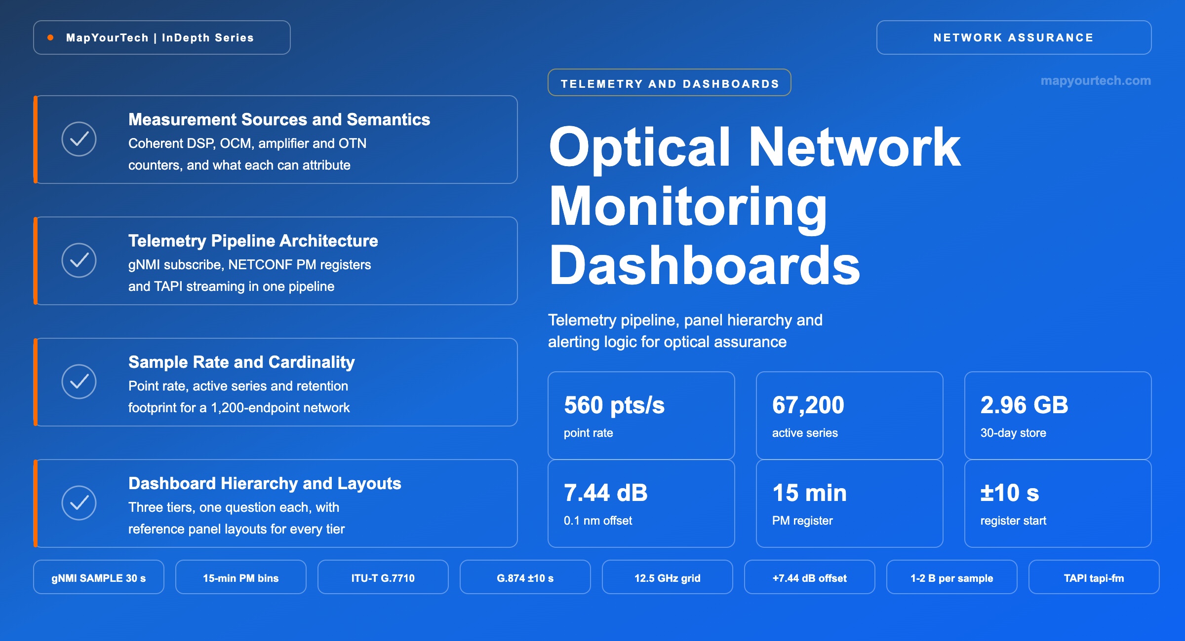
- Separate the four optical measurement sources — coherent DSP, optical channel monitor, amplifier telemetry and OTN counters — by what each one can and cannot attribute.
- Place gNMI subscriptions, NETCONF 15-minute registers and TAPI streaming in one collection architecture, per Figure 1.
- Compute telemetry point rate, active series cardinality and retention footprint — 560 points/s and 2.96 GB per 30 days for the worked reference network.
- Convert pre-FEC BER to Q-factor and receiver SNR to 0.1 nm OSNR before plotting them together — 7.44 dB of offset at 69.4 GBd.
- Build the three-tier panel hierarchy — network overview, lightpath drill-down and span element view — from the reference layouts in Figures 4 to 6.
- Configure a gNMI collector, a PromQL margin rule and a TAPI streaming client from the paste-ready examples in Section 6.
- Instrument the pipeline itself against the four collector KPIs in Section 7, so a silent collector cannot look like a healthy network.
- Select a collector, time-series store and visualization layer against the comparison matrix in Section 9.
1. Introduction
An optical line system already measures almost everything an operations team needs. A coherent receiver reports pre-forward-error-correction bit error rate (pre-FEC BER), chromatic dispersion, differential group delay and received signal-to-noise ratio (SNR) as a by-product of digital signal processing (DSP) it performs anyway. An optical channel monitor (OCM) in a reconfigurable optical add-drop multiplexer (ROADM) degree reports per-channel power and noise floor across the band. Every erbium-doped fiber amplifier (EDFA) reports input power, output power, gain and pump laser bias current. The data exists. What usually does not exist is a path from those registers to a screen where an engineer can see, in one view, that a 400 Gb/s service crossing six spans has lost 1.4 dB of margin over three weeks.
That gap is an integration problem rather than a measurement problem, and it has grown wider as networks disaggregated. A single-vendor network came with a single-vendor element management system whose performance screens were adequate because they only had one data model to render. An open line system carrying third-party coherent pluggables has at least three data models in play — OpenROADM for the line system, OpenConfig for the terminal device, and whatever the router platform exposes for the host — and no vendor screen that spans them. The dashboard becomes the operator's own artifact, assembled from streams the operator subscribes to and stores.
The problem this article addresses is narrower than observability in general. It is the specific engineering of an optical monitoring surface: which registers to subscribe to, at what cadence, how many time series that produces, how to store them without the retention cost growing faster than the network, how to convert quantities that are measured in different reference bandwidths before plotting them on one axis, and how to lay out panels so that the first screen answers a question rather than displaying a wall of gauges. Three reference layouts are given in Section 5, and the collector configurations behind them in Section 6.
The commercial context is a shift from polling to subscription. gNMI (the gRPC Network Management Interface) inverted the collection model: the device pushes typed updates on change or on a sample interval, and the collector parses protocol buffers rather than walking an object identifier tree. Streaming telemetry is reported by the OpenConfig community and by vendors to reach roughly a hundredfold the resolution of Simple Network Management Protocol (SNMP) polling — a vendor-and-operator claim rather than a standard-specified figure, and one that matters mainly because it changes what a dashboard can show. At 30-second cadence, a power transient that lasts 90 seconds appears as three points. At 15-minute registers, it appears as a slightly elevated average or not at all.
Standards work has caught up with the practice. TAPI v2.4.0 unified the alarm and performance-monitoring structures that earlier versions carried separately in notification and streaming, so a controller's northbound interface can now deliver alarms and PM through one model. OpenROADM device models expose current and historical PM lists in 15-minute, 24-hour and untimed bins over NETCONF. TM Forum publishes TMF642 Alarm Management and TMF628 Performance Management as Open APIs for the operations support system boundary above that. The pieces for a standards-based monitoring stack are in place; assembling them is the work.
Takeaway: The measurements already exist in the line system and the coherent receiver. Building a monitoring dashboard is an exercise in subscription design, data normalization and panel hierarchy — not in adding instrumentation.
2. Measurement Sources and Data Semantics
An optical monitoring dashboard draws on four measurement sources, and they differ in what they can attribute. Confusing them is the most common reason a dashboard shows a degradation without pointing at its cause.
2.1 Coherent Receiver DSP Telemetry
The coherent receiver is the densest instrument in the network. Its DSP already estimates chromatic dispersion to compensate it, tracks polarization state to demultiplex it, and counts corrected and uncorrected bits inside the FEC decoder. Reading those estimates costs nothing extra. Pre-FEC BER is the primary health metric because it moves continuously and monotonically with received signal quality, while post-FEC BER stays at zero until the link is nearly failing and then collapses. Received SNR, reported per polarization or as an aggregate, is the receiver's own estimate of the electrical signal-to-noise ratio after equalization, and it therefore includes transceiver implementation penalties that an optical measurement does not see.
The attribution limit matters: a receiver metric describes the end-to-end path as the receiver experiences it. It cannot tell you which span degraded. It is the alarm bell, not the fault locator. The relationship between these quantities is worked through in the article on OSNR, BER and Q-factor as link performance parameters.
2.2 Optical Channel Monitor and Optical Spectrum Measurement
An OCM in a ROADM degree sweeps the band and reports per-channel centre frequency, power and, where the channel spacing allows it, an interpolated noise floor from which in-band optical signal-to-noise ratio (OSNR) is estimated. Its value is spatial: a per-degree OCM reading localizes a power or noise change to a node. Its limits are equally specific. In-band OSNR estimation by spectral interpolation degrades once channels are packed tightly enough that the inter-channel floor is no longer noise-only, and an OCM reports optical condition without any knowledge of the receiver's tolerance to it. Monitoring practice for this layer is covered in the discussion of optical performance monitoring architectures.
Read the Full Analysis with Premium
The remaining 88% of this article — the design numbers, trade-offs and field guidance — is part of MapYourTech Premium, along with the full premium library, courses and professional tools.
You May Also Like
-
Free
-
August 22, 2026

-
Premium
-
August 22, 2026
-
Premium
-
August 22, 2026