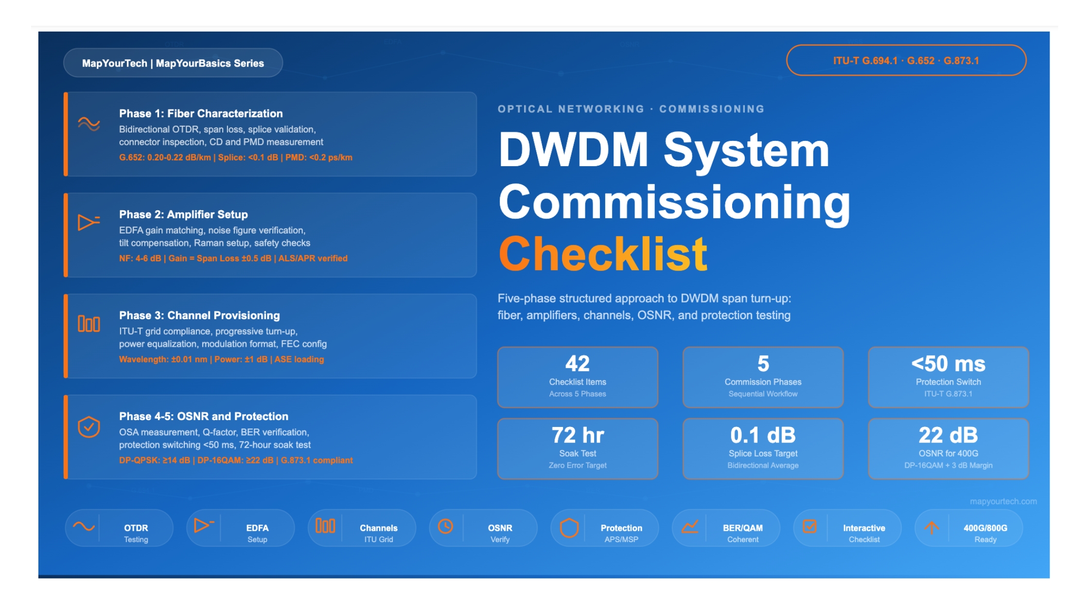

DWDM System Commissioning Checklist
A Practical Quick-Reference Guide for Commissioning New DWDM Spans: Fiber Characterization, Amplifier Setup, Channel Provisioning, OSNR Verification, and Protection Testing
1. Introduction
Commissioning a new Dense Wavelength Division Multiplexing (DWDM) span is among the most critical activities in optical network deployment. A poorly commissioned span introduces latent performance issues that compound over time, degrade signal quality across the entire wavelength plan, and can result in costly service-affecting failures months or years after initial turn-up. Conversely, a well-executed commissioning process establishes reliable performance baselines, validates design assumptions, and ensures the span operates within its engineered margins from day one.
This guide presents a structured, phase-based commissioning checklist covering the five essential stages of DWDM span turn-up: fiber characterization, amplifier setup, channel provisioning, OSNR verification, and protection testing. Each phase builds on the results of the previous one, forming a logical sequence that experienced optical engineers can follow as a practical quick-reference during field deployment. The content is anchored in industry standards from ITU-T, IEEE, and established engineering practice, with numerical thresholds and formulas drawn from real-world deployment guidelines.
Whether commissioning a metro ring with 80 km spans or a long-haul corridor stretching over 1,000 km with multiple amplifier sites, the fundamental process remains the same. What changes are the specific thresholds, the amplification strategy (EDFA, Raman, or hybrid), and the modulation format requirements of the coherent transponders being deployed. This guide addresses all these variables with practical worked examples and decision frameworks.
Figure 1: The five-phase DWDM commissioning workflow with key deliverables at each stage. Each phase must be completed and documented before advancing to the next.
2. Phase 1 -- Fiber Characterization
Fiber characterization is the foundational step in any DWDM commissioning process. The physical fiber plant determines the fundamental performance limits of the entire optical system. No amount of sophisticated DSP or amplification can overcome a fiber infrastructure that falls outside its design parameters. This phase validates that the installed fiber meets the specifications assumed during the link engineering process.
2.1 OTDR Testing
Optical Time-Domain Reflectometry (OTDR) provides a comprehensive map of the fiber span, identifying every splice, connector, bend, and anomaly along the route. The OTDR works by injecting optical pulses into the fiber and measuring the intensity and timing of backscattered and reflected light. The resulting trace reveals the fiber's attenuation profile, splice locations and losses, connector reflections, and any unexpected events such as macrobends or damaged sections.
For single-mode fiber, the true splice loss at any point must be determined by the bidirectional average of OTDR readings, as recommended by ITU-T standards. A one-way OTDR measurement should not be used as actual splice loss because Mode Field Diameter (MFD) tolerances and other intrinsic parameter differences between fibers can cause significant measurement errors. In single-mode fiber, single-direction OTDR readings at a splice can appear either positive or negative, potentially masking a problematic splice or flagging a good one.
OTDR Testing Checklist
2.2 Span Loss Verification
Beyond OTDR testing, end-to-end span loss must be verified using an optical power source and power meter (the insertion loss method). This provides the definitive span loss value used for amplifier configuration and link budget calculations. The measured span loss must be compared against the engineered design value, and any discrepancy greater than 1 dB should trigger investigation.
-- Span Loss Calculation --

Span Loss (dB) = Fiber Attenuation + Splice Losses + Connector Losses + Safety Margin

Where:
  Fiber Attenuation = α × L       α = 0.20-0.22 dB/km @ 1550 nm (G.652)
  Splice Loss       = Nsplices × αsplice  Typical: 0.05-0.1 dB per fusion splice
  Connector Loss    = Nconnectors × αconn  Typical: 0.3-0.5 dB per mated pair
  Safety Margin     = 1-3 dB     Accounts for aging, repairs, environmental factors

-- Worked Example: 80 km span --
  Fiber: 80 km × 0.21 dB/km       = 16.80 dB
  Splices: 8 × 0.08 dB           =  0.64 dB
  Connectors: 4 × 0.35 dB       =  1.40 dB
  Margin:                          =  2.00 dB
  -------------------------------------
  Total Engineered Span Loss      = 20.84 dB
2.3 Chromatic Dispersion and PMD Testing
For coherent systems operating at 100G and above, modern DSP compensates for chromatic dispersion (CD) electronically, eliminating the need for dispersion compensating fiber (DCF) in most deployments. However, CD testing remains valuable for establishing a baseline and for legacy 10G direct-detect channels that may share the same fiber. Standard single-mode fiber (G.652) exhibits approximately 17 ps/(nm·km) of dispersion at 1550 nm.
Polarization Mode Dispersion (PMD) testing is more critical for qualifying fiber for high-speed coherent transmission. PMD arises from birefringence in the fiber and causes differential group delay (DGD) between polarization states. The total PMD of a link combining fiber and components is calculated as follows:
-- Total Link PMD Calculation --

PMDTOTAL = √( PMDF2 × L + Σ PMDCi2 )

Where:
  PMDF   = Fiber PMD coefficient (ps/√km)   Typical: ≤ 0.1 ps/√km for modern fiber
  L      = Fiber length (km)
  PMDCi = PMD of the i-th optical component (ps)

-- Example: 400 km link, 4 components @ 0.6 ps each --
  PMDTOTAL = √( (0.1)2 × 400 + 4 × (0.6)2 )
           = √( 4.0 + 1.44 )
           = √( 5.44 )
           = 2.33 ps  < 2.5 ps limit for 40G systems
Practical Note: For coherent 100G/200G/400G systems, PMD tolerance is significantly higher than for legacy direct-detect systems. Modern coherent DSP can compensate for PMD values exceeding 50 ps with negligible penalty. However, PMD measurement remains good practice to establish a baseline and to identify any fiber sections with unusually high PMD that may indicate installation problems.
| Parameter | Unit | Acceptance Threshold | Action if Failed |
|---|---|---|---|
| Fiber Attenuation @ 1550 nm | dB/km | ≤ 0.22 (G.652), ≤ 0.23 (G.655) | Investigate for macrobends; re-route if needed |
| Fiber Attenuation @ 1310 nm | dB/km | ≤ 0.35 (G.652) | Compare against specification sheet |
| Fusion Splice Loss (bidirectional avg.) | dB | ≤ 0.1 (target), ≤ 0.3 (max per ITU-T G.671) | Re-splice; any visible spike requires re-splice |
| Connector Insertion Loss | dB | ≤ 0.3 (per mated pair, active alignment) | Clean and re-inspect; replace connector if persistent |
| Connector Return Loss (APC) | dB | ≥ 45 | Clean end-face; inspect for damage with fiber microscope |
| PMD Coefficient | ps/√km | ≤ 0.2 (recommended); ≤ 0.5 (maximum) | Identify high-PMD sections; may need fiber replacement |
| Chromatic Dispersion @ 1550 nm | ps/(nm·km) | ≤ 18 (G.652); verify coherent DSP range | Baseline recording; DCM if legacy 10G channels present |
| Optical Return Loss (total link) | dB | ≥ 26 | Locate reflective events via OTDR; clean or re-terminate |
Table 1: Fiber Characterization Acceptance Thresholds -- parameters, limits, and corrective actions for DWDM span commissioning.
3. Phase 2 -- Amplifier Setup and Commissioning
Once the fiber plant passes characterization, attention turns to the optical amplifiers that will compensate for span losses. EDFA commissioning establishes the gain, noise figure, output power, and tilt compensation parameters that directly determine the system's OSNR budget and, by extension, the maximum achievable reach and capacity. In systems using Raman amplification or hybrid EDFA/Raman configurations, additional parameters including pump power levels and counter-propagating pump wavelength alignment must be verified.
3.1 EDFA Configuration and Gain Verification
EDFAs in DWDM systems typically operate in one of two modes: automatic gain control (AGC) or constant output power mode. For inline amplifiers on a new commissioning, AGC mode tied to the measured span loss is the standard approach. The EDFA gain should be set to match the span loss of the preceding fiber section, such that the per-channel power at the amplifier output matches the design target.
The gain of an EDFA is a function of pump power and the length of the erbium-doped fiber. In practical systems, EDFAs operate in gain saturation so that output power remains relatively constant independent of input power variations. However, the gain shape (the spectral profile of gain across the C-band or L-band) varies with operating gain, producing what is called gain tilt. This tilt must be compensated to maintain uniform per-channel power across the wavelength plan.
EDFA Commissioning Checklist
3.2 OSNR Contribution Calculation
Each EDFA introduces ASE noise that degrades the OSNR. Understanding the OSNR contribution of each amplifier in the chain is essential for predicting end-to-end link performance. The OSNR at the output of a single EDFA can be calculated from the amplifier's noise figure and the input signal power.
-- Single-Amplifier OSNR Calculation --

OSNRdB = Pin - NF - 10 log10(h × v × Bref) - 10 log10(G)

Simplified (0.1 nm reference bandwidth at 1550 nm):
OSNRdB = 58 + Pin - NF

Where:
  Pin    = Per-channel input power (dBm)
  NF     = Amplifier noise figure (dB)
  58     = Constant for 0.1 nm reference BW at 1550 nm: -10 log(h×v×Δv)

-- Cascaded OSNR for N amplifiers --
1/OSNRtotal = Σ (1 / OSNRi)   for i = 1 to N (linear domain)

-- Example: 5 spans, Pin = -15 dBm, NF = 5.5 dB --
  OSNR per amp = 58 + (-15) - 5.5 = 37.5 dB
  Cascaded OSNR (5 identical amps) = 37.5 - 10 log(5) = 37.5 - 7.0 = 30.5 dB
3.3 Raman and Hybrid Amplifier Setup
For spans exceeding 25-28 dB of loss, or where the EDFA-only OSNR budget is insufficient, Raman amplification provides distributed gain along the fiber itself. Raman pumps are counter-propagating (launched from the downstream amplifier site back toward the upstream site), and the Raman gain depends on the pump power, pump wavelength, and fiber type.
When commissioning Raman amplifiers, the gain deviation from the ATR (Automatic Test Report) values provided in the amplifier's IDProm must be verified against the actual fiber type deployed. Different fiber types (G.652, G.655 LEAF, G.654) produce different Raman gain coefficients, and the ATR tables are specific to each fiber type. The operator must confirm the correct fiber type is configured in the NMS before enabling Raman pumps.
Safety Consideration: Always verify that automatic laser shutdown (ALS) and automatic power reduction (APR) mechanisms are operational before enabling high-power Raman pumps. Raman pump powers typically range from 500 mW to 2 W, and exposure to these power levels presents a serious eye safety hazard. Follow IEC 60825-2 laser safety procedures during all amplifier commissioning activities.
Figure 2: A five-span DWDM link showing EDFA placement with hybrid Raman amplification on the high-loss span. OSA measurement at the receiver terminal validates end-to-end OSNR.
4. Phase 3 -- Channel Provisioning
With the amplifier chain commissioned and baselined, the next phase involves provisioning optical channels. This includes configuring transponders to the correct ITU-T grid wavelengths, verifying per-channel power levels at key measurement points, and confirming that the channel plan matches the network design documentation. Channel provisioning follows a methodical sequence: start with a single test channel, expand to a subset, and finally bring up the full wavelength plan.
4.1 Wavelength Plan and ITU-T Grid
DWDM systems operate on the ITU-T G.694.1 frequency grid. The standard defines channel center frequencies with spacings of 12.5 GHz, 25 GHz, 50 GHz, and 100 GHz. For flex-grid systems supporting super-channels (400G and beyond), the 12.5 GHz granularity allows arbitrary spectral slot widths in multiples of 12.5 GHz. The C-band extends from approximately 191.3 THz (1567.13 nm) to 196.1 THz (1528.77 nm), supporting up to 96 channels at 50 GHz spacing or 48 channels at 100 GHz spacing.
Channel Provisioning Checklist
4.2 Power Budget Verification
The received power at each channel must fall within the receiver's acceptable input power range. Too little power degrades OSNR; too much power can cause receiver overload or trigger nonlinear effects in the fiber. The power budget validation ensures that the system operates within its design margins.
-- Power Budget Formula --

PRX = PTX - Σ(Losses) + Gamp - M

Where:
  PRX      = Received power per channel (dBm)
  PTX      = Per-channel transmit power (dBm)
  Losses   = Total losses: fiber + connectors + MUX/DEMUX + splices
  Gamp     = Total amplifier gain across the link (dB)
  M        = System margin (typically 3-5 dB)

-- Worked Example: 3-span 100G QPSK link --
  PTX per channel:       0 dBm
  MUX insertion loss:      -5 dB
  Span 1 loss (80 km):     -18 dB    EDFA 1 gain: +18 dB
  Span 2 loss (80 km):     -18 dB    EDFA 2 gain: +18 dB
  Span 3 loss (80 km):     -18 dB    Pre-amp gain: +22 dB
  DEMUX insertion loss:    -5 dB
  System margin:           -3 dB

  PRX = 0 - 5 - 18 + 18 - 18 + 18 - 18 + 22 - 5 - 3 = -9 dBm
  Typical coherent Rx range: 0 to -18 dBm -- PASS
5. Phase 4 -- OSNR Verification
OSNR verification is the most critical quality-of-service check during DWDM commissioning. OSNR directly determines the achievable bit error rate (BER) and, consequently, whether the system will meet its capacity and reliability targets. OSNR is measured using an optical spectrum analyzer (OSA) at the receiver terminal, before the DEMUX, to capture the per-channel signal-to-noise ratio across the entire wavelength plan.
5.1 OSNR Measurement Methodology
OSNR is defined as the ratio of signal power to noise power within a standard reference bandwidth, typically 0.1 nm (12.5 GHz). The OSA measures both the signal peak power and the noise floor between channels. For coherent systems with closely spaced channels (50 GHz or less), interpolation techniques may be needed to estimate the noise power underneath the signal, since the noise floor between channels may not represent the noise at the signal wavelength accurately.
In submarine and open cable systems, OSNR characterization has been standardized using ASE noise loading techniques. Noise channels can be generated using an ASE source followed by a wavelength selective switch (WSS), greatly simplifying the test setup compared to using multiple laser sources. ASE noise loading also eliminates polarization-related measurement artifacts. As noted in ITU-T G.977.1 for open cable systems, OSNR measurements should be performed across the full usable bandwidth with power profiles representative of traffic conditions.
OSNR Verification Checklist
5.2 OSNR Requirements by Modulation Format
| Modulation Format | Line Rate | Minimum OSNR (0.1 nm ref) | Recommended Margin | Typical Operating OSNR |
|---|---|---|---|---|
| DP-QPSK | 100G | ~9.8 dB (at BER = 3.8 x 10⁻³) | 3 dB | ≥ 14 dB |
| DP-QPSK | 200G (64 GBd) | ~12 dB | 3 dB | ≥ 16 dB |
| DP-8QAM | 300G | ~15 dB | 3 dB | ≥ 19 dB |
| DP-16QAM | 200G (32 GBd) | ~16.5 dB | 3 dB | ≥ 20 dB |
| DP-16QAM | 400G (64 GBd) | ~18 dB | 3 dB | ≥ 22 dB |
| DP-64QAM | 600G+ | ~24 dB | 3 dB | ≥ 27 dB |
Table 2: OSNR requirements by modulation format. Minimum OSNR values represent the theoretical threshold at standard SD-FEC BER limits. The recommended margin accounts for implementation penalties, aging, and nonlinear effects.
5.3 OSNR Degradation Across Distance
The following chart illustrates how end-to-end OSNR decreases with increasing number of amplified spans, assuming typical EDFA parameters. The horizontal lines represent the minimum required OSNR for different modulation formats, showing the maximum reach achievable for each.
Figure 3: End-to-end OSNR vs. number of spans for a typical EDFA chain (per-channel input power: -15 dBm, NF: 5.5 dB). Horizontal thresholds show minimum OSNR for common modulation formats including 3 dB system margin.
6. Phase 5 -- Protection Testing
The final commissioning phase validates that protection and restoration mechanisms function correctly under both planned and unplanned failure conditions. Protection testing confirms that the network can recover from fiber cuts, equipment failures, and software faults within the switchover time requirements defined in the service level agreement (SLA). For DWDM systems, this includes both optical layer protection (such as 1+1 fiber protection or ROADM-based mesh restoration) and OTN layer protection (SNCP/SNCi at the path level).
6.1 Protection Switching Tests
Protection Testing Checklist
6.2 Protection Switching Time Breakdown
-- Protection Switching Time Calculation --

Tswitch = Tdetect + Tnotify + Tconfig

Where:
  Tdetect = Fault detection time       Typically 5-10 ms (hardware-based LOS detection)
  Tnotify = Notification propagation   Typically 5-15 ms (depends on ring circumference)
  Tconfig = Path configuration time    Typically 10-25 ms (switch activation + settling)

-- Performance targets --
  1+1 Protection:    < 50 ms   (per ITU-T G.873.1)
  ROADM Restoration: < 200 ms  (typical for WSS-based switching)
  Mesh Restoration:  < 2 sec   (depends on path computation time)
7. Commissioning Quick-Reference Summary
Phase 1: Fiber
Bidirectional OTDR at 1310/1550 nm. End-to-end loss verification. Splice loss < 0.1 dB. Connector IL < 0.3 dB, ORL > 45 dB (APC). CD and PMD baseline recording. All traces documented.
Phase 2: Amplifiers
EDFA gain = span loss. NF ≤ 6 dB. Gain flatness ±1 dB. Tilt compensation configured. ALS/APR safety verified. Raman pumps aligned to correct fiber type. ATR data recorded.
Phase 3: Channels
ITU-T grid compliance. Wavelength accuracy ±0.01 nm. Progressive channel turn-up. Power flatness < 1 dB. ASE loading for partial fill. FEC mode configured. Modulation format verified.
Phase 4: OSNR
OSA-based per-channel OSNR. Meets modulation format threshold + 3 dB margin. Pre-FEC BER below FEC limit. Post-FEC error-free. Q-factor documented. Measured vs. design comparison.
Phase 5: Protection
Protection switchover < 50 ms. Hitless for 1+1. Reversion tested. Forced/manual switch commands verified. NMS alarms validated. 72-hour soak test with zero errors.
Final Acceptance
All five phases PASS. Performance baselines archived. Soak test documentation complete. As-built drawings updated. Customer acceptance document signed and countersigned.
8. Essential Test Equipment
| Equipment | Primary Use | Key Specifications | Commissioning Phase |
|---|---|---|---|
| OTDR | Fiber loss profiling, splice/event identification | Dynamic range ≥ 40 dB, multi-wavelength (1310/1550/1625 nm) | Phase 1 |
| Optical Power Meter | End-to-end loss, per-channel power | Range: +10 to -50 dBm, accuracy ±0.2 dB | Phase 1, 3, 4 |
| Light Source (calibrated) | Insertion loss measurement | Stable output ±0.05 dB, 1310/1550 nm | Phase 1 |
| Optical Spectrum Analyzer (OSA) | OSNR, channel power, spectral analysis | Resolution ≤ 0.02 nm, dynamic range ≥ 50 dB | Phase 2, 3, 4 |
| Fiber Inspection Microscope | Connector end-face inspection | 400x magnification, IEC 61300-3-35 pass/fail | Phase 1 |
| PMD Analyzer | Differential group delay measurement | Accuracy ±0.1 ps, range 0-100 ps | Phase 1 |
| CD Analyzer | Chromatic dispersion profiling | Range: 1250-1650 nm, accuracy ±5% | Phase 1 |
| BER Test Set / Traffic Generator | Error rate and traffic verification | Pattern generation, error counting, protocol-aware | Phase 4, 5 |
Table 3: Essential test equipment for DWDM commissioning with recommended specifications and the commissioning phases where each instrument is required.
9. Troubleshooting Common Commissioning Issues
Even with rigorous procedures, commissioning teams frequently encounter issues that require systematic diagnosis. The following table summarizes the most common problems observed during DWDM commissioning, along with their probable causes and recommended corrective actions.
| Symptom | Probable Cause | Corrective Action |
|---|---|---|
| Span loss exceeds design by > 2 dB | Dirty or damaged connectors, bad splice, macrobend | OTDR trace analysis to localize the excess loss; clean/re-terminate connectors; re-splice if needed |
| EDFA not reaching target gain | Pump laser degradation, incorrect gain mode, input power below minimum | Check pump current vs. threshold; verify gain mode setting; confirm input power above EDFA minimum |
| OSNR lower than predicted | Higher-than-expected span loss, NF degradation, additional unaccounted loss element | Re-measure all span losses; verify EDFA NF from ATR data; check for overlooked attenuators or patch cords |
| Significant power tilt across band | Incorrect EDFA tilt setting, SRS effect, gain shape mismatch | Recalculate required tilt compensation; adjust EDFA tilt parameter; verify DGE operation if equipped |
| Pre-FEC BER above threshold on select channels | Low OSNR on edge channels, nonlinear penalty, adjacent channel crosstalk | Adjust per-channel power; reduce launch power if nonlinear effects suspected; check channel spacing |
| Protection switch takes > 50 ms | Software configuration error, slow fault detection, congested control plane | Verify protection group configuration; check hardware detection thresholds; review control plane loading |
| Wavelength drift alarm on transponder | Temperature control issue, locker circuit fault | Check transponder temperature; verify wavelength locker operation; replace module if persistent |
Table 4: Common commissioning issues, root causes, and resolution steps.
10. Future Directions in DWDM Commissioning
DWDM commissioning practices continue to evolve alongside advances in optical networking technology. Several trends are reshaping how operators commission and validate new spans.
Automated Commissioning and Zero-Touch Provisioning: As of 2025, the industry is moving toward highly automated commissioning workflows. Modern DWDM platforms integrate with SDN controllers that can discover the physical topology, measure span losses through pilot tones, and automatically configure EDFA gains and tilt parameters without manual intervention. Wavelength-tunable pluggable transceivers with self-tuning capabilities further reduce provisioning complexity by automatically scanning for the correct channel on the mux/demux filter, eliminating manual wavelength configuration and reducing human error during turn-up.
IP-over-DWDM and Open Line Systems: The growing adoption of coherent pluggables (400ZR, 400ZR+, and emerging 800ZR interfaces) directly in routers is changing the commissioning paradigm. In these architectures, the optical line system (OLS) operates independently of the transponders, and commissioning focuses on validating the open line system's spectral characteristics (GSNR, power profile) rather than end-to-end transponder-based measurements. Multi-vendor interoperability testing becomes a key part of the commissioning process in these open architectures.
C+L Band Expansion: As operators expand from C-band-only systems to combined C+L band operation to double fiber capacity, commissioning procedures must account for inter-band effects, particularly Stimulated Raman Scattering (SRS) that transfers power from the C-band to the L-band. Tilt management becomes more complex, and separate amplifier chains for each band require independent commissioning followed by joint inter-band optimization.
GSNR-Based Acceptance: For open cable architectures, particularly in submarine systems, the industry is adopting Generalized Signal-to-Noise Ratio (GSNR) as the primary commissioning metric. GSNR decouples the optical link performance from the transponder, providing a modulation-independent view of the transmission line's quality. This approach, already standardized for submarine open cables, is expected to extend to terrestrial open line systems as multi-vendor deployments become more common.
References
[1] ITU-T Recommendation G.694.1 -- Spectral grids for WDM applications: DWDM frequency grid.
[2] ITU-T Recommendation G.671 -- Transmission characteristics of optical components and subsystems.
[3] ITU-T Recommendation G.652 -- Characteristics of a single-mode optical fibre and cable.
[4] ITU-T Recommendation G.977.1 -- Characteristics of optically amplified optical fibre submarine cable systems.
[5] ITU-T Recommendation G.873.1 -- Optical transport network: Linear protection.
[6] ITU-T Recommendation G.709 -- Interfaces for the optical transport network.
[7] IEC 60825-2 -- Safety of laser products: Safety of optical fibre communication systems.
[8] IEC 61300-3-35 -- Fibre optic interconnecting devices and passive components: Visual inspection of fibre optic connector end faces.
[9] Sanjay Yadav, "Optical Network Communications: An Engineer's Perspective" -- Bridge the Gap Between Theory and Practice in Optical Networking.
Developed by MapYourTech Team
For educational purposes in Optical Networking Communications Technologies
Note: This guide is based on industry standards, best practices, and real-world implementation experiences. Specific implementations may vary based on equipment vendors, network topology, and regulatory requirements. Always consult with qualified network engineers and follow vendor documentation for actual deployments.
Feedback Welcome: If you have any suggestions, corrections, or improvements to propose, please feel free to write to us at [email protected]