
Fiber Dispersion Slope:
Impact on Wideband DWDM Performance
A comprehensive engineering guide to dispersion slope (ps/nm²/km), its effect on multi-band DWDM channels, slope-compensating DCF design, and how coherent DSP eliminates residual slope penalties.
Introduction
Chromatic dispersion is one of the most studied impairments in optical fiber transmission. Engineers designing DWDM systems are familiar with the dispersion coefficient D, expressed in ps/(nm·km), which describes how different wavelengths travel at different group velocities through the fiber. For a single channel at a fixed wavelength, compensating dispersion is straightforward: match the accumulated positive dispersion of the transmission fiber with an equivalent length of negative-dispersion compensating fiber (DCF), and the pulse arrives at the receiver undistorted.
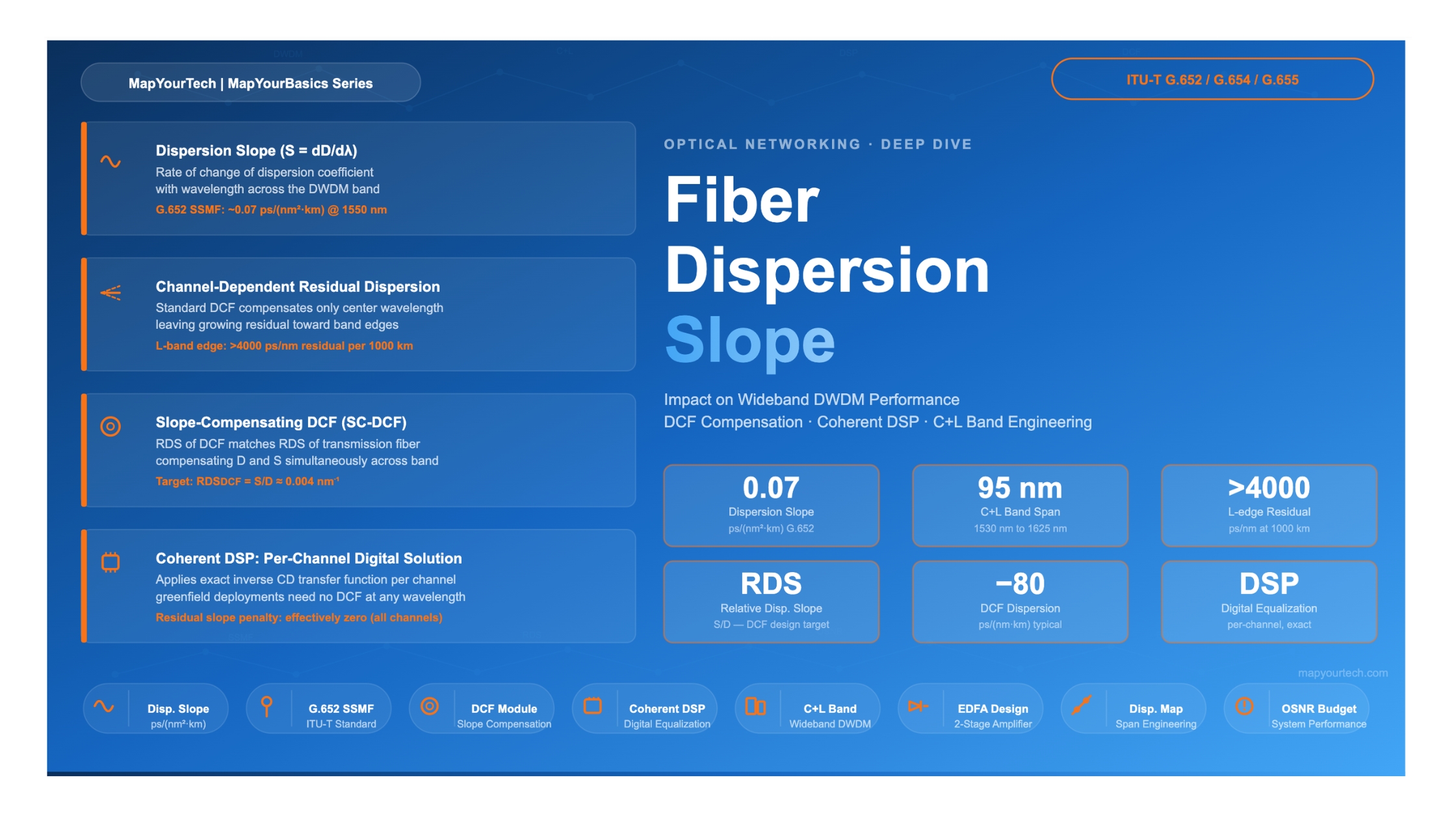
Wideband DWDM systems, however, do not carry a single channel. A fully loaded C-band system carries 80 or more channels spanning 1530–1565 nm. Add an L-band (1565–1625 nm) and the spectral occupancy nearly doubles. Across this span — roughly 10 THz in combined C+L — the dispersion coefficient itself changes with wavelength. That change is the dispersion slope, denoted S and expressed in ps/(nm²·km). It is the derivative of D with respect to wavelength.
Dispersion slope matters because a compensation module optimized for one wavelength — typically the center of the band — will leave progressively larger residual dispersion at channels near the band edges. In a C-band-only system this residual is manageable. In a C+L system spanning more than 90 nm, or in an ultra-long-haul system accumulating many thousands of ps/nm of dispersion per span, uncompensated slope produces per-channel residual dispersion values that exceed the tolerance of 100G and 400G coherent transceivers relying on direct detection or limited DSP.
This article examines dispersion slope from first principles, explains how it accumulates differently across the channel grid, describes how slope-compensating DCF modules are designed, and explains why coherent DSP has fundamentally changed the engineering approach to residual slope management.
Fundamental Principles of Dispersion and Dispersion Slope
2.1 Chromatic Dispersion: A Recap
Chromatic dispersion in single-mode fiber arises from two contributions: material dispersion, caused by the wavelength dependence of the refractive index of silica glass, and waveguide dispersion, caused by the distribution of light between the core and cladding at a given wavelength. The total chromatic dispersion coefficient D(λ) is the derivative of group delay τg with respect to wavelength:
/* Dispersion coefficient definition */
D(λ) = dτg / dλ   [ps/(nm·km)]

Where:
τg  = group delay per unit length (ps/km)
 λ  = wavelength (nm)

Equivalently in terms of propagation constant β:
D(λ) = −(2πc / λ²) · β(2)

Where:
 c     = speed of light in vacuum (≈ 3 × 10⁸ m/s)
 β(2) = group velocity dispersion (GVD) coefficient (ps²/km)
For ITU-T G.652 standard single-mode fiber (SSMF), D at 1550 nm is approximately +17 ps/(nm·km). The positive sign means longer wavelengths travel faster — they have a shorter group delay — so the trailing edge of a pulse (redder components) arrives before its leading edge (bluer components), broadening the pulse in time.
2.2 Dispersion Slope: Definition and Physical Origin
The dispersion slope S is the rate of change of D with wavelength. It quantifies how dispersion varies across the optical spectrum:
/* Dispersion slope definition */
S(λ) = dD / dλ   [ps/(nm²·km)]

For G.652 SSMF at 1550 nm — typical value:
S ≈ +0.06 to +0.09 ps/(nm²·km)

For G.655 NZDSF at 1550 nm — typical value:
S ≈ +0.04 to +0.11 ps/(nm²·km)   (large relative slope)

For submarine G.654-class low-loss fiber:
S ≤ +0.07 ps/(nm²·km)
The physical origin of dispersion slope lies in both material and waveguide contributions. The material dispersion of silica glass has a characteristic curvature in its D(λ) curve; the zero-dispersion wavelength near 1310 nm marks where material and waveguide contributions cancel. Moving toward 1550 nm, D rises following a roughly linear trend, giving a positive slope. Waveguide contributions add a secondary component that depends on fiber design: fibers engineered to have a specific dispersion value at 1550 nm (like NZDSF) inevitably acquire a different slope profile than SSMF, as bending the D(λ) curve to hit a target dispersion value at one wavelength pulls the slope away from its natural silica value.
Modern submarine fibers designed for digital coherent transmission — where large effective area and low loss are the primary design goals rather than dispersion control — tend to have dispersion values of +18 to +23 ps/(nm·km) and slopes of +0.07 ps/(nm²·km) or lower at 1550 nm, because their designs stay close to the natural silica material dispersion profile.
2.3 Relative Dispersion Slope (RDS)
The relative dispersion slope (RDS) is a dimensionless figure of merit that describes how much of the dispersion coefficient is "consumed" per nanometer of wavelength deviation. It provides a compact way to compare fibers and DCF modules:
/* Relative Dispersion Slope */
RDS = S / D   [1/nm]

Example — G.652 SSMF at 1550 nm:
RDS = 0.07 ps/(nm²·km)  /  17 ps/(nm·km)
     ≈ 0.0041 nm⁻¹

For perfect slope compensation, the DCF must match:
RDSDCF = RDStransmission fiber
When the RDS of the DCF module matches the RDS of the transmission fiber, the ratio of dispersion-slope compensation equals the ratio of dispersion compensation, and residual dispersion is equalized to zero across all channels simultaneously. This is the design target for a wideband slope-compensating DCF module.
How Dispersion Slope Degrades Wideband DWDM Systems
3.1 Channel-Dependent Residual Dispersion
Consider a 100-km span of G.652 SSMF with D = 17 ps/(nm·km) and S = 0.07 ps/(nm²·km). A DCF module compensates dispersion exactly at the center wavelength λ0 = 1550 nm. For channels at a wavelength offset Δλ from center, the residual dispersion per span is:
/* Residual dispersion at channel offset Δλ */
Dresidual(Δλ) = S · L · Δλ   [ps/nm]

Where:
 S  = dispersion slope of transmission fiber  (ps/nm²/km)
 L  = span length (km)
 Δλ = wavelength offset from compensation center (nm)

Example — C-band edge channel (Δλ = +17.5 nm from 1547.5 nm center):
 Dresidual = 0.07 × 100 × 17.5 = +122.5 ps/nm per span

After 10 spans (1000 km):
 Accumulated residual = 0.07 × 1000 × 17.5 = 1225 ps/nm

C+L combined, edge channel (Δλ = +45 nm at L-band edge):
 Dresidual = 0.07 × 1000 × 45 = 3150 ps/nm
Design implication: For a 1000 km link with no slope compensation, channels at the L-band edge accumulate over 3000 ps/nm of residual dispersion when S = 0.07 ps/(nm²·km). The dispersion tolerance of a direct-detection 10G channel is approximately ±1000 ps/nm per ITU-T G.691. Even a 100G coherent channel, though far more tolerant via DSP, can face performance penalties from unmanaged residual slope at this scale.
3.2 Channel-Specific Residual Dispersion — Worked Example
The table below shows how residual dispersion per 1000 km span varies across DWDM channels for G.652 SSMF with S = 0.07 ps/(nm²·km), compensated at 1550 nm, without slope compensation:
| Channel (nm) | Band | Δλ from 1550 nm (nm) | D at channel (ps/(nm·km)) | Residual dispersion @ 1000 km (ps/nm) | Impact |
|---|---|---|---|---|---|
| 1530 | C-band edge | −20 | 15.6 | −1400 | Near tolerance limit (10G) |
| 1540 | C-band | −10 | 16.3 | −700 | Within tolerance (10G/100G) |
| 1550 | C-band center | 0 | 17.0 | 0 | Perfectly compensated |
| 1560 | C/L boundary | +10 | 17.7 | +700 | Within tolerance (100G) |
| 1580 | L-band | +30 | 19.1 | +2100 | Exceeds 10G tolerance |
| 1600 | L-band | +50 | 20.5 | +3500 | Significant penalty (100G) |
| 1620 | L-band edge | +70 | 21.9 | +4900 | Severe — requires correction |
Figure 1: Per-Channel Residual Dispersion vs Wavelength (1000 km, no slope compensation)
Figure 1: Residual dispersion accumulates symmetrically around the compensation center wavelength. C-band channels remain within ±1400 ps/nm; L-band edge channels exceed 4000 ps/nm after 1000 km — well beyond direct-detection tolerances and challenging for coherent systems at high modulation orders.
3.3 Multi-Span Accumulation and the Dispersion Map
In a DWDM system, a dispersion compensator (PDC or DCF) is typically placed at the mid-stage of each inline amplifier, or at the transmit and receive terminals. The dispersion map — the plot of cumulative dispersion versus distance — shows the dispersion accumulated at each wavelength as a function of span position.
A PDC can exactly compensate for chromatic dispersion at one wavelength, but it typically cannot exactly compensate at all other wavelengths simultaneously. The difference in residual dispersion between channels can be reduced in long-haul systems by applying dispersion compensation and dispersion slope compensation together. Without slope compensation, the dispersion map fans out progressively with each span: channels near the band center accumulate little residual, while channels at the band edges accumulate increasing residual with each span traversed.
This fanning behavior has important consequences. After N spans, the worst-case residual at the band edge is N times the single-span residual. For a 20-span ultra-long-haul system, residuals that appeared manageable after one span become catastrophic after twenty.
Single-Span View
Residual dispersion at each channel is proportional to S × L × Δλ. Edge channels see the most residual per span. DCF optimized for center wavelength leaves a linear tilt in residual vs. wavelength.
Multi-Span Accumulation
Residuals add coherently across spans (same sign for same Δλ). After N spans, edge-channel residual = N × (S × L_span × Δλ). Ultra-long-haul links see residuals exceeding thousands of ps/nm.
Dispersion Map Fanning
The dispersion map fans out like an open book: center channels stay near zero, edge channels diverge. Slope compensation collapses this fan, keeping all channels near zero residual simultaneously.
Slope-Compensating Dispersion Compensating Fiber (DCF)
4.1 Standard DCF: The Single-Wavelength Solution
Standard DCF is a specialty fiber engineered to have a large negative dispersion coefficient — typically around −80 ps/(nm·km) — achieved by designing a small, highly guiding core that shifts the zero-dispersion wavelength well outside the operating band. A short length of DCF thus compensates the dispersion of a much longer span of SSMF. The condition for perfect single-channel compensation is:
/* Standard DCF compensation condition (single wavelength) */
DSMF × LSMF + DDCF × LDCF = 0

Typical values:
 DSMF  = +17 ps/(nm·km)   LSMF = 100 km  → accumulated = +1700 ps/nm
 DDCF  = −80 ps/(nm·km)   LDCF = ?

 LDCF = 1700 / 80 = 21.25 km

So ~21 km of standard DCF compensates 100 km of G.652 SSMF at center wavelength.
However, standard DCF was designed to minimize insertion loss for a given dispersion value, not to match the dispersion slope of the transmission fiber. The RDS of standard DCF (approximately 0.003 nm−1) typically does not match the RDS of SSMF (approximately 0.004 nm−1), so residual slope remains after compensation. For C-band-only systems at 10G rates, this mismatch was acceptable. For wideband systems at 100G and beyond, it is not.
4.2 Slope-Compensating DCF: Design Principles
A slope-compensating DCF (sometimes called wideband DCF or dispersion-slope-compensating module, DSCM) is designed so that its RDS matches the RDS of the transmission fiber. This means that when you compensate the accumulated dispersion at the center wavelength, you also compensate the accumulated slope across the entire operating band simultaneously.
/* Slope compensation condition (all wavelengths simultaneously) */

Condition 1 — Dispersion compensation at center wavelength:
DSMF(λ0) × LSMF + DDCF(λ0) × LDCF = 0

Condition 2 — Slope compensation (RDS matching):
SSMF / DSMF = SDCF / DDCF   → RDSSMF = RDSDCF

Equivalently:
SSMF × LSMF + SDCF × LDCF = 0

Residual dispersion at any channel offset Δλ (when both conditions are met):
Dresidual(Δλ) = 0   for all Δλ
Meeting both conditions requires that the DCF have a large negative dispersion and a large negative slope, such that their ratio equals the ratio of the transmission fiber. For G.652 SSMF, this means the DCF must have an RDS of approximately 0.0041 nm−1. Standard DCF typically has an RDS around 0.003 nm−1, so achieving full slope matching requires a specially designed fiber structure.
4.3 Fiber Design for Slope Matching
Engineering a fiber with a large RDS — meaning a large slope-to-dispersion ratio — requires managing both material and waveguide contributions carefully. Several design approaches achieve this:
Dual-core or W-profile designs: A ring-shaped refractive index profile (W-profile or dual-core design) introduces additional waveguide dispersion that can be shaped to produce a large negative slope alongside a large negative dispersion coefficient. These designs typically have small effective areas (around 20–30 µm²) due to the strongly confining core geometry needed to produce high waveguide dispersion.
Segmented-core designs: Multiple concentric core regions of different refractive indices allow finer control of both dispersion and slope. The trade-off is manufacturing complexity and the difficulty of maintaining consistent parameters along long fiber lengths.
The small effective area of slope-compensating DCF introduces a key operational trade-off: high optical power density at the fiber core increases nonlinear effects — particularly self-phase modulation (SPM) and cross-phase modulation (XPM). Systems using DCF modules must limit the optical power entering the DCF or insert the DCF at the mid-stage of a two-stage amplifier, where the signal power is lower. The two-stage amplifier architecture — with a pre-amplifier, then the DCF, then a booster amplifier — is the standard approach in 10G and legacy systems. The booster stage compensates the DCF insertion loss (typically 6–10 dB) without degrading the optical signal-to-noise ratio (OSNR), since the pre-amplifier has already boosted the signal well above the noise floor.
4.4 DCF Module Placement and Residual Tolerance
| Parameter | Standard DCF | Slope-Compensating DCF | Unit |
|---|---|---|---|
| Dispersion coefficient D | −80 to −100 | −80 to −120 | ps/(nm·km) |
| Dispersion slope S | −0.25 to −0.30 | −0.35 to −0.50 | ps/(nm²·km) |
| RDS (S/D) | ~0.003 | ~0.004 (matches G.652) | nm⁻¹ |
| Effective area Aeff | ~20–30 | ~15–25 | µm² |
| Insertion loss per module | 5–8 | 7–12 | dB |
| Operating bandwidth | C-band (35 nm) | C+L-band (95+ nm) | nm |
| Target application | Single-band 10G–40G | Wideband 40G–100G | — |
Figure 2: Residual Dispersion Comparison — Standard DCF vs Slope-Compensating DCF (1000 km)
Figure 2: Standard DCF (blue) leaves a linear residual dispersion tilt across the band, growing toward the edges. Slope-compensating DCF (green) holds residual near zero across the full C+L band. The fan-out with standard DCF exceeds ±3000 ps/nm at L-band edges over 1000 km.
4.5 Practical Limitations of Passive Slope Compensation
Even with carefully designed slope-compensating DCF, achieving perfect compensation across the full C+L band over many spans presents practical challenges. Fiber manufacturing tolerances introduce span-to-span variation in D and S. The DCF modules themselves have manufacturing tolerances. Over a long-haul route assembled from multiple fiber segments from different manufacturing batches, the accumulated residual dispersion at any given channel is not exactly zero — it follows a statistical distribution whose width grows with route length.
Statistical analysis shows that for a 400 km link built with G.652 fiber and five dispersion compensators, the combined residual dispersion of fiber plus compensators for the C-band (1530–1565 nm) spans a range of approximately ±600 ps/nm at a 3σ confidence level. The limit for 10 Gbit/s transmission with respect to chromatic dispersion alone is approximately 1000 ps/nm per ITU-T G.691. This leaves a working margin, but leaves little room for additional penalties in a fully engineered OSNR budget.
For wideband C+L systems, the statistical challenge is compounded by the larger Δλ values involved. Tunable dispersion compensators (TDCs) can fine-tune per-channel residual dispersion after installation, providing per-channel adjustment that static DCF modules cannot offer. Tunable fiber Bragg gratings (FBGs) are one approach to TDC implementation. Alternatively — and this is the dominant approach in modern systems — residual dispersion is handled entirely in the electronic domain using coherent DSP.
Coherent DSP: Full Digital Management of Residual Dispersion Slope
5.1 The Coherent Receiver Architecture
The introduction of digital coherent receivers in commercial DWDM systems — beginning around 2010 and now ubiquitous in 100G, 400G, and 800G transponders — fundamentally changed how engineers approach dispersion management. A coherent receiver preserves both the amplitude and phase of the received optical field by mixing the signal with a narrow-linewidth local oscillator (LO) in a 90-degree optical hybrid. The output of the four balanced photodetectors yields in-phase (I) and quadrature (Q) components for both polarizations, providing the complete complex field representation of the received signal.
With the full complex field available, the digital signal processor in the coherent receiver can apply an inverse transfer function of the fiber channel — including chromatic dispersion, polarization mode dispersion (PMD), and other linear impairments — entirely in the digital domain. Dispersion compensation becomes a filtering problem.
5.2 Digital Chromatic Dispersion Compensation
Chromatic dispersion is a deterministic, static linear impairment. For a given fiber link of fixed length and dispersion coefficient, the accumulated chromatic dispersion at any channel wavelength is constant over time. This makes it ideally suited to a static finite impulse response (FIR) filter or a frequency-domain equalizer implemented once and updated only when the network topology changes.
The transfer function of chromatic dispersion in the frequency domain is:
/* Transfer function of chromatic dispersion (frequency domain) */
HCD(z, ω) = exp( j · β2 · ω² · z / 2 )

Where:
 β2 = GVD parameter (ps²/km) = −D · λ² / (2πc)
 ω  = angular frequency offset from carrier
 z  = fiber length (km)

To compensate, the DSP applies the conjugate transfer function:
Heq(z, ω) = exp( −j · β2 · ω² · z / 2 )

After equalization, the impulse response is restored to near-ideal.

Dispersion tolerance of coherent systems — approximate rule of thumb:
 Tolerable CD ≈ 1 / (Ds · Bs²)

Where:
 Ds = dispersion at the channel wavelength
 Bs = symbol rate

For 32 GBaud coherent, tolerable CD with full DSP equalization:
Effectively unlimited — DSP handles all accumulated dispersion
(filter length scales with accumulated CD × symbol rate²)
For short impulse responses — low accumulated dispersion — a time-domain FIR filter approach is preferred. For systems with high accumulated CD, such as long-haul links where the impulse response can span thousands of symbols, frequency-domain equalizers implemented with the fast Fourier transform (FFT) using an overlap-and-save method are more computationally efficient. Modern coherent ASIC implementations use frequency-domain CD equalization as the static stage, followed by shorter adaptive butterfly equalizers for dynamic impairments such as PMD and polarization rotation.
5.3 Slope Compensation: The DSP Advantage
The critical advantage of coherent DSP over passive DCF for dispersion slope management is channel-by-channel independence. Each coherent transponder processes only its own channel. The DSP knows the exact carrier wavelength of its channel, and therefore the exact accumulated dispersion — including any residual from imperfect slope compensation — at that wavelength. It can apply the precise equalizer tap coefficients needed to invert the exact dispersion value at its channel, regardless of what other channels experience.
This means that residual dispersion slope — the differential dispersion between channels that passive DCF fails to eliminate — is completely transparent to a coherent DSP. A channel at the L-band edge experiencing 3000 ps/nm of residual dispersion is equalized with the same quality as a C-band center channel experiencing 10 ps/nm, provided the DSP has enough filter taps to span the impulse response length corresponding to 3000 ps/nm at the deployed symbol rate.
Practical note on DSP filter length: The impulse response duration for a given accumulated CD (in ps/nm) and symbol rate Rs (in GBaud) scales as CD × Rs² / c. At 32 GBaud, 1000 ps/nm of accumulated dispersion corresponds to an impulse response of approximately 20 symbol periods. At 3000 ps/nm, this extends to roughly 60 symbol periods. Modern ASIC implementations accommodate accumulated CD values far exceeding these figures. Some commercial implementations handle over 100,000 ps/nm of accumulated CD, far more than any terrestrial C+L system can accumulate, making DCF entirely unnecessary in greenfield coherent deployments.
5.4 DSP Architecture for Dispersion Equalization
The equalization function in a digital coherent receiver partitions into two stages. The first stage is a static equalizer implementing the matched filter and the CD compensation filter (hCD). Since CD changes slowly — it is constant until the optical path changes — this filter is computed once and held static between path changes. It is typically implemented using FFT-based fast convolution for efficiency.
The second stage is a dynamic equalizer: a set of four adaptive FIR filters forming the 2×2 butterfly structure (hxx, hxy, hyx, hyy). This stage compensates for polarization rotation, PMD, and residual dynamic effects, updated in real time using error-based adaptation algorithms such as the Constant Modulus Algorithm (CMA) for constant-envelope formats or decision-directed algorithms for higher-order QAM.
The partitioning is not arbitrary: it reflects the very different time scales and filter lengths involved. The CD filter for a 1000 km link at 32 GBaud may require hundreds of taps, while the polarization butterfly filter requires only tens of taps but must update on millisecond time scales. Separating them allows each to be implemented in the most efficient manner.
Figure 3: Accumulated Dispersion Handling — Coherent DSP vs Passive DCF (per channel, 1000 km)
Figure 3: Coherent DSP eliminates per-channel residual dispersion exactly regardless of accumulated value. Passive DCF can only compensate a fixed dispersion value per module, leaving slope-induced residual untouched. The gap between the two approaches widens toward the L-band and over longer routes.
5.5 Implications for System Design: DCF-Free Architectures
The consequence of coherent DSP's ability to handle arbitrary accumulated CD on a per-channel basis is profound for system architecture. Modern greenfield coherent DWDM networks — particularly those deploying 100G, 400G, or 800G coherent channels — are designed without any inline DCF. This approach, sometimes called dispersion-unmanaged (DU) transmission, eliminates DCF modules from the amplifier mid-stage entirely.
The advantages of removing DCF are substantial. DCF modules add insertion loss (typically 6–10 dB per module), which must be compensated by additional EDFA gain, consuming pump power and adding amplified spontaneous emission (ASE) noise. DCF's small effective area concentrates optical power in a small core, exacerbating nonlinear effects such as SPM and XPM. Removing DCF reduces the total link insertion loss per span, allows lower launch powers, and significantly reduces nonlinear impairments. Research has shown that systems without DCF exhibit less nonlinear penalty than systems with DCF, because DCF creates concentrated nonlinear interaction zones within the link.
Modern design guideline: For new coherent DWDM deployments using 100G, 400G, or 800G coherent transponders, DCF is not required. DSP handles all accumulated CD and residual slope. The dispersion map is no longer a design constraint. Amplifier mid-stages can be simplified, span loss budgets improve, and nonlinear performance is enhanced. DCF remains relevant primarily in legacy systems running direct-detection 10G channels alongside coherent channels, where the 10G channels still require passive dispersion management.
Fiber Type Comparison: Slope Characteristics Across the ITU-T Portfolio
Different fiber standards have significantly different dispersion slopes, with important implications for DWDM system design and the magnitude of slope compensation required.
| Fiber Standard | D @ 1550 nm (ps/(nm·km)) | S @ 1550 nm (ps/(nm²·km)) | RDS (nm⁻¹) | Aeff (µm²) | Key Application |
|---|---|---|---|---|---|
| G.652 SSMF | +17 | +0.06–0.09 | ~0.004 | ~80 | Terrestrial terrestrial long-haul, metro |
| G.654 PSCF (large core) | +20 to +22 | ≤+0.07 | ~0.003–0.004 | 110–150 | Submarine, ultra-long-haul |
| G.655 NZDSF | −14 to −4 (low D) | +0.04–0.11 | ~0.006–0.010 | ~50–72 | WDM with reduced FWM |
| G.653 DSF | ≈0 at 1550 nm | +0.07–0.09 | very large | ~50 | Legacy single-channel (not WDM) |
| Typical DCF | −80 to −100 | −0.25 to −0.30 | ~0.003 | ~20–30 | C-band compensation |
| Slope-compensating DCF | −80 to −120 | −0.35 to −0.50 | ~0.004 (matched) | ~15–25 | C+L wideband compensation |
6.1 Why NZDSF Presented Special Slope Challenges
Non-zero dispersion-shifted fiber (G.655 NZDSF) was designed to solve the four-wave mixing (FWM) problem of DSF: by positioning the zero-dispersion wavelength outside the EDFA amplification band (outside 1525–1620 nm), NZDSF ensured that channels in the operating window always experienced some dispersion, breaking the phase-matching condition for FWM. However, NZDSF's engineered dispersion profile came with a larger relative dispersion slope than SSMF.
The relative dispersion slope of NZDSF can be two to three times that of G.652 SSMF, making it significantly harder to compensate with DCF modules. The large RDS of NZDSF means that a standard DCF optimized for center-wavelength compensation leaves more residual slope across the band per span. Submarine systems using NZDSF in the early 2000s found this slope difficult to manage over multi-thousand-kilometer routes, contributing to the eventual adoption of large-core pure-silica-core fibers (similar to G.654) for modern submarine deployments, where the dispersion stays close to the natural silica glass profile and the slope is controlled.
Practical Applications and Implementation Strategies
7.1 Legacy 10G DWDM: Dispersion Map Engineering
In legacy direct-detection 10G DWDM systems, dispersion management is an explicit design discipline. The engineer must construct a dispersion map — a plan for how cumulative dispersion evolves along the link — that keeps every channel's accumulated dispersion within the receiver's tolerance window at every point in the network.
For a direct-detection 10G channel, the chromatic dispersion tolerance is typically specified as approximately ±1000 ps/nm. The C-band statistical analysis for G.652 fiber and standard compensators indicates that the combined residual dispersion over a 400 km link with 5 compensators lies within approximately ±600 ps/nm at the 3σ level. This leaves a working margin for the C-band. Adding L-band channels with standard DCF would push residuals at the L-band edge well beyond ±1000 ps/nm, which is why legacy 10G systems were generally restricted to C-band operation.
Deploying slope-compensating DCF modules — or a combination of standard DCF at the inline amplifiers and slope-compensating modules at the terminal or at specific mid-route sites — was the engineering solution for wideband 10G systems, where both C and L bands were required simultaneously.
7.2 Mixed 10G/100G Networks: The Hybrid Challenge
Many operators have hybrid networks carrying legacy direct-detection 10G channels alongside coherent 100G channels on the same fiber. This presents a specific design challenge: the 10G channels still require passive dispersion management via DCF, while the 100G coherent channels would actually perform better without DCF (due to DCF's nonlinear impairment). The DCF modules required for the 10G channels impose nonlinear penalties on the 100G coherent channels sharing the fiber.
The standard solution in hybrid networks is to retain the existing DCF infrastructure for 10G channel compatibility, and to accept slightly elevated nonlinear penalties for the 100G coherent channels, which the coherent DSP partially mitigates. As 10G channels are migrated off the network over time, operators gradually remove DCF modules from inline amplifiers, transitioning to a fully DCF-free architecture as 100G and above coherent channels take over.
7.3 C+L Wideband Systems: Design Considerations
Modern C+L band systems using coherent transponders approach dispersion slope management from a different starting point than legacy systems. Because coherent DSP handles residual dispersion per channel, the system designer's primary concern shifts from "how do I compensate slope across the band" to "how do I ensure the amplifiers, gain equalization, and stimulated Raman scattering (SRS) power tilt are managed correctly across the wider spectrum."
The SRS effect transfers power from shorter (C-band) channels to longer (L-band) channels at a rate that grows with the total optical power and the bandwidth of the channel comb. In a C+L system spanning approximately 90 nm, this SRS-induced power tilt is significant and must be actively equalized. This is a distinct challenge from dispersion slope management, though both arise from the same wideband spectral occupancy.
Dispersion slope remains a secondary concern in C+L coherent systems primarily in two contexts: first, when verifying that the coherent ASIC's CD equalization range is sufficient for the worst-case accumulated CD at the L-band edge channels over the planned route length, and second, when designing the dispersion map for any legacy direct-detection channels that may coexist in the system.
Greenfield Coherent (C-band)
No DCF required. DSP handles all accumulated CD at center and edge channels. Span loss budget improves. Design focus: OSNR, nonlinear noise, gain flatness.
C+L Coherent Expansion
DSP per channel handles residual slope independently. Design focus: SRS tilt management, L-band EDFA design, per-channel gain equalization, OSNR over wider band.
Legacy 10G Upgrade Path
Retain DCF for 10G channels. Assess coherent ASIC CD range vs route length. Plan DCF removal milestones as 10G channels migrate to 100G coherent.
Performance Optimization and Trade-offs
8.1 The Dispersion Map as a Nonlinear Tool
In direct-detection and early coherent systems, the dispersion map was used not only to keep residual dispersion within tolerance but also as a tool to manage nonlinear impairments. Maintaining a non-zero local dispersion at all points along the link reduces the efficiency of FWM by preventing phase-matched four-wave mixing between channels. Over-compensation (running with slightly positive or slightly negative residual dispersion in each span before correction at the amplifier) was a common technique to suppress nonlinear interactions.
Coherent systems with DSP have largely decoupled dispersion management from nonlinear management. The dispersion map need not be optimized for nonlinear suppression because the DSP handles the dispersion, and nonlinear effects (which remain uncompensated by linear DSP) are addressed separately through launch power optimization and, in advanced systems, digital back-propagation or nonlinear compensation algorithms.
8.2 DSP Filter Length and ASIC Resource Constraints
While coherent DSP can in principle handle any accumulated CD, there is a practical resource constraint: the number of DSP filter taps is finite, bounded by the ASIC silicon area and power budget. At very high symbol rates and very large accumulated CD, the CD equalization filter must be implemented with a large number of FFT bins in the frequency-domain equalizer. ASIC implementations for commercial coherent modules are designed with a maximum supported CD value that covers the intended deployment scenarios with margin.
As symbol rates increase toward 100 GBaud and beyond for future 800G and 1.6T transponders, the filter length required for a given accumulated CD scales quadratically with symbol rate. This places tighter constraints on ASIC CD equalization range at very high baud rates, potentially bringing dispersion slope back into relevance for the longest routes at the highest baud rates, particularly when L-band channels at edge wavelengths are combined with ultra-long reach requirements.
8.3 Quantifying Residual Slope Penalty in Coherent Systems
Even though coherent DSP compensates residual slope exactly in the linear domain, there is an indirect penalty mechanism: equalization-enhanced phase noise (EEPN). When the CD filter is very long — corresponding to high accumulated CD — the laser phase noise (LPN) from the transmitter laser is spread in time by the dispersion and then partially correlated with the LPN at the receiver. The interaction of large dispersion with finite laser linewidth creates an excess noise contribution that grows with accumulated CD and laser linewidth.
EEPN is modeled as a noise growing with the product of accumulated CD and the square of the symbol rate. For typical narrow-linewidth lasers used in coherent transceivers (linewidth below 100 kHz), EEPN is negligible at C-band accumulated dispersions (up to approximately 30,000 ps/nm for a 2000 km C-band link). It becomes non-negligible for very long routes at L-band edge wavelengths, where accumulated dispersion at 1620 nm can exceed 50,000 ps/nm over a 2000 km link, motivating precise accounting of L-band edge CD in long-haul network design.
Future Directions
The trajectory of DWDM system design points toward ever-wider spectral occupancy, higher baud rates, and smarter DSP implementations. Several trends are shaping how dispersion slope will be handled in next-generation systems.
S-band expansion: Some research and early commercial systems are exploring the S-band (1460–1530 nm) as an additional capacity layer beyond C+L. The S-band sits on the other side of the 1530 nm EDFA absorption edge, requiring different amplification technologies such as thulium-doped fiber amplifiers (TDFAs) or Raman amplification. Dispersion at S-band wavelengths is substantially different from C and L band values on the same fiber — for G.652 SSMF, D at 1490 nm is approximately +6–8 ps/(nm·km), versus +17 ps/(nm·km) at 1550 nm — and the dispersion slope across a combined S+C+L system spanning 160 nm is far larger in absolute accumulated terms than for C+L alone. DSP-based coherent systems handle this per-channel, but the ASIC CD equalization range specification becomes a critical parameter for S-band deployments.
Higher baud rates: Transponder baud rates have risen from 32 GBaud toward 100 GBaud and beyond. At these symbol rates, the impulse response duration per unit of accumulated CD is proportionally shorter (fewer symbol periods per ps/nm), but the total number of filter taps required for a given absolute CD grows as the square of the baud rate. ASIC designers must weigh CD equalization range against power consumption in future generations.
Machine learning for dispersion tracking: Networks operate over fiber that changes slowly with temperature and mechanical stress. Adaptive DSP algorithms that can track slow changes in accumulated CD without manual intervention are increasingly important as systems scale in channel count and span length. Machine learning approaches that predict CD changes from environmental monitoring data — linking temperature sensor readings to expected dispersion shifts — are emerging as tools for reducing the overhead of periodic CD re-calibration in field-deployed networks.
Submarine C+L expansion: While submarine systems have historically used C-band only, C+L band transmission is a leading technology option for increasing cable capacity without new fiber deployment. Submarine C+L requires redesigned repeaters with dual-band EDFA stages and careful management of both SRS and dispersion slope across the combined band. Modern submarine fibers with slopes of ≤ 0.07 ps/(nm²·km) and large effective areas facilitate this expansion, with coherent DSP handling per-channel residual slope across the full bandwidth.
Conclusion
Dispersion slope — the rate of change of chromatic dispersion with wavelength, expressed in ps/(nm²·km) — is not a second-order concern in DWDM system engineering. For any system spanning more than a narrow slice of the optical spectrum, slope causes each channel to accumulate a different amount of dispersion, with the differential growing linearly with the wavelength offset from the compensation center and accumulating span by span across a multi-span route.
For direct-detection systems operating across wide spectral bands, slope-compensating DCF modules that match the relative dispersion slope (RDS) of the transmission fiber are the passive engineering tool for containing per-channel residual dispersion. These modules require careful fiber design to achieve the required RDS while managing effective area and insertion loss trade-offs, and they must be positioned in the amplifier mid-stage architecture to avoid excess nonlinear penalties.
Coherent DSP has transformed slope management from a passive optical engineering problem into an essentially solved digital signal processing problem. Each coherent transponder's CD equalizer applies the exact inverse transfer function for its own channel's accumulated dispersion — including all residual slope from imperfect passive compensation or from entirely DCF-free architectures. This per-channel digital exactness is something no passive optical module can match. For greenfield coherent deployments, the engineering question about dispersion slope has largely become: does the ASIC's CD equalization range cover the worst-case accumulated dispersion at the L-band edge for the planned route length? In modern implementations, the answer is almost always yes.
As DWDM systems expand into C+L and eventually C+L+S bands, and as baud rates rise toward 100 GBaud and beyond, the interaction between accumulated CD at extreme wavelengths and DSP resource constraints will keep dispersion slope relevant as a design parameter. Understanding its physical origin, its channel-dependent accumulation behavior, the engineering principles of passive slope compensation, and the capabilities of digital equalization gives network engineers the complete toolkit needed to design and operate wideband optical transport systems at any capacity level.
Summary — Main Points
- Dispersion slope S (ps/nm²/km) = dD/dλ. For G.652 SSMF, S ≈ +0.07 ps/(nm²·km) at 1550 nm. It causes different DWDM channels to accumulate different amounts of dispersion, with the differential growing toward band edges.
- In a 1000 km C+L system with no slope compensation, L-band edge channels can accumulate over 4000 ps/nm of residual dispersion — well beyond direct-detection tolerances and significant even for coherent transceivers at high modulation orders.
- Slope-compensating DCF is designed so that its relative dispersion slope (RDS = S/D) matches that of the transmission fiber, compensating both dispersion and slope simultaneously across the full band. This requires specialty fiber with large negative slope and small effective area.
- Coherent DSP applies the exact per-channel inverse transfer function for accumulated CD at each channel's specific wavelength, providing perfect digital slope compensation independently for every channel — something passive optics cannot match.
- Modern greenfield coherent DWDM systems are designed without DCF (dispersion-unmanaged), relying entirely on coherent DSP. Removing DCF reduces insertion loss, improves OSNR, and reduces nonlinear impairments from DCF's small effective area.
References
- ITU-T Recommendation G.652 – Characteristics of a single-mode optical fibre and cable.
- ITU-T Recommendation G.654 – Characteristics of a cut-off shifted single-mode optical fibre and cable.
- ITU-T Recommendation G.655 – Characteristics of a non-zero dispersion-shifted single-mode optical fibre and cable.
- ITU-T Recommendation G.691 – Optical interfaces for single-channel STM-64 and other SDH systems with optical amplifiers.
- ITU-T Recommendation G.694.1 – Spectral grids for WDM applications: DWDM frequency grid.
- TR-OFCS (2015-07) – Technical Report on Optical Fiber Communication Systems, ITU-T G-series Recommendations Supplement 39.
- Sanjay Yadav, "Optical Network Communications: An Engineer's Perspective" – Bridge the Gap Between Theory and Practice in Optical Networking.
- Undersea Fiber Communication Systems, Elsevier, 2025 – Section 12: Submarine fiber evolution and chromatic dispersion in coherent systems.
- Ip E., Kahn J.M., "Digital equalization of chromatic dispersion and polarization mode dispersion," Journal of Lightwave Technology, 2007.
- Savory S.J., "Digital filters for coherent optical receivers," Optics Express, 2008.
Developed by MapYourTech Team
For educational purposes in Optical Networking Communications Technologies
Note: This guide is based on industry standards, best practices, and real-world implementation experiences. Specific implementations may vary based on equipment vendors, network topology, and regulatory requirements. Always consult with qualified network engineers and follow vendor documentation for actual deployments.
Feedback Welcome: If you have suggestions, corrections, or improvements to propose, please write to us at [email protected]