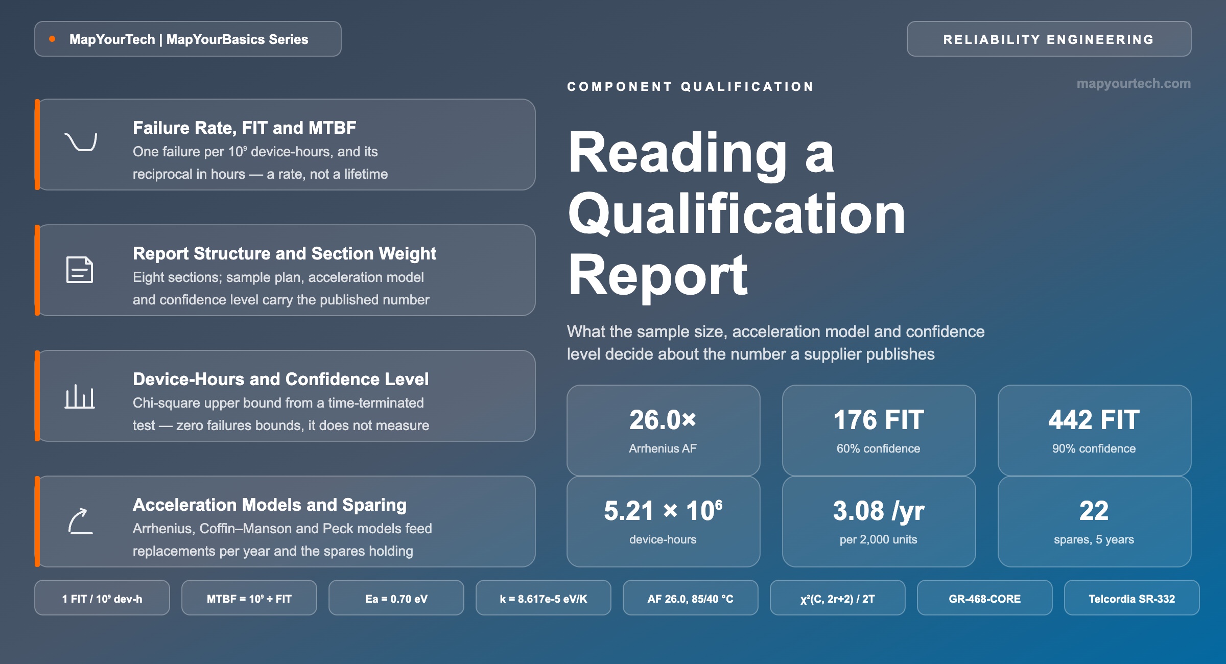
Reading a Component Qualification Report
What the sample size, the acceleration model, the stress conditions and the confidence level decide about the number a supplier publishes.
A test condition omitted is a specification withdrawn.
1. Introduction
A supplier reliability figure arrives as one number. A coherent pluggable datasheet gives 176 FIT; a line card quotes a mean time between failures of 5.7 million hours; a passive optical component states a 25-year service life. Each of those is the output of a statistical procedure, and the procedure has four inputs that the number itself does not carry: how many units were tested, for how many hours, under what stress, and at what confidence level the result was bounded. Change any one of those and the same test data produces a different published figure, sometimes by a factor of three.
That is not a criticism of suppliers. Telcordia SR-332 asks explicitly that a published MTBF or FIT figure be accompanied by its method and its assumptions, including the operating temperature, the electrical stress, the environmental and quality factors, and the confidence level (standard-specified, Telcordia SR-332). A report that states all of them is doing what the procedure asks. A report that states only the answer has left the reader to guess the inputs.
This article walks one qualification report structure, states which sections carry the load, and gives the three questions to put to a supplier when a section is thin. The reference case throughout is a coherent pluggable module qualified under Telcordia GR-468-CORE: 100 units, 2,000 h of powered life test at 85 °C, zero failures, referred to a 40 °C use condition. Every calculator in the article opens on that case, so the number in the prose and the number on screen agree. The scope is component and module qualification for terrestrial optical transport hardware; it stops where system-level modelling begins, which is covered separately in the MapYourTech treatment of optical network architecture design for maximum availability.
2. Failure Rate, FIT and MTBF Definitions
Failure rate is the number of failures a population of components produces per unit of operating time, expressed in FIT — one FIT equals one failure per 109 device-hours. Mean time between failures is its reciprocal in hours. Both describe the flat middle of a component's life curve, after early failures have been screened out and before wearout begins, and neither describes how long a part lasts.
Distinctions From the Adjacent Quantities
Five pairs get conflated, and each confusion changes a decision. Failure rate against FIT: these are the same quantity in different units, FIT being failures per 109 device-hours rather than failures per hour. FIT against MTBF: also the same information, related by a reciprocal, so a report quoting both is quoting one measurement twice. MTBF against MTTF: mean time between failures applies to a repairable item that returns to service after a card swap, mean time to failure to a non-repairable one that is discarded, and an optical module is treated either way depending on whether the operator repairs or replaces. MTBF against service life: 5.7 million hours is 648 years, and no pluggable lasts 648 years — the figure describes a rate inside the flat region, while service life is set by the wearout mechanisms that GR-468-CORE aging tests are designed to find. Point estimate against upper confidence bound: the same test data yields a best estimate and a bound, and a report that does not say which one it published has left out half the answer.
Units and Conversion
MTBF (h) = 109 ÷ λ (FIT) and λ (FIT) = 109 ÷ MTBF (h)
Where:
- λ — failure rate in FIT, one FIT being one failure per 109 device-hours. Typical qualified module values range from tens to a few thousand FIT.
- MTBF — mean time between failures in hours. Divide by 8,760 for years.
- Device-hours — units multiplied by hours of operation, the denominator both quantities are built on.
Taking the reference case result of 176 FIT: MTBF = 109 ÷ 176 = 5.68 × 10⁶ h, which is 648 years. Read as a rate it says that 10,000 such modules produce about 15.4 failures per year of continuous operation. Read as a lifetime it says nothing at all, because the module's service life is bounded by laser and package wearout mechanisms that the constant-rate model does not contain.
Takeaway: FIT and MTBF are one measurement in two units, and both are rates rather than lifetimes. Every number that follows in a qualification report is a statement about the flat region of the hazard-rate curve, so a report that never shows where that region ends has bounded the rate without bounding the service life.
3. Report Structure and Section Weight
A qualification report follows the same skeleton whatever the component, because the underlying reliability assurance programme does. Telcordia GR-468-CORE sets out that programme for optoelectronic devices — supplier approval, device qualification, lot-to-lot controls, failure analysis feedback, and change control — and GR-1221-CORE does the same for passive optical components (standard-specified, Telcordia). The report is the evidence package for one branch of that programme, and its sections do not carry equal weight.
| Report section | What it constrains | Symptom when thin |
|---|---|---|
| Device identity and configuration | Which build, package, wavelength plan and firmware the data applies to | Data quoted for a family, not the part number being bought |
| Sample plan and lot traceability | Sample size and how many production lots the units came from | All units from one lot, so lot-to-lot variation is untested |
| Stress conditions and duration | Temperature, humidity, bias, cycle count and hours applied | Test named but conditions absent, so acceleration cannot be checked |
| Failure criterion | The parameter drift that ends a unit's life on test | “No failures” with no stated pass limit |
| Failure analysis | Root cause and mechanism for every unit that failed | Failures counted but not attributed, so no read-across to the field |
| Acceleration model | Model form and activation energy converting test to field hours | Field-equivalent hours stated with no model behind them |
| Rate calculation | Device-hours, failure count and confidence level | A FIT number with no confidence level attached |
| Change control | Which changes trigger a product change notification and requalification | Silent process or supplier changes after the report was issued |
Three of those sections do most of the work. The sample plan sets the denominator, the acceleration model sets the multiplier on that denominator, and the confidence level sets how much of the resulting margin the supplier chose to keep. The remaining sections are the audit trail that lets a reader believe the three. This mirrors the discipline applied in coherent optical transponder test and measurement, where a tolerance figure quoted without its measurement conditions is not comparable with anyone else's.
Standards currency
GR-468-CORE Issue 2 was ratified in 2004 and its module-level test set — mechanical integrity, non-powered environmental stress, powered environmental stress — predates non-hermetic packaging, silicon photonics and PAM4 signalling. The International Photonics and Electronics Committee has published a Carrier-grade Optical Modules Reliability Implementation Agreement that adds environmental tests the older document does not carry, including dust, airborne contaminant and corrosion testing for carrier environments with weaker sulfur and dust control than data centres (standard-specified, IPEC). A report that cites GR-468-CORE alone is complete against that document and silent on those mechanisms.
Takeaway: Sample plan, acceleration model and confidence level determine the published number; every other section exists so that a reader can check those three. A report is thin where one of the three is stated as a result rather than as a method.
4. Sample Size, Device-Hours and Confidence Level
Zero failures on test does not produce a failure rate of zero. It produces an upper bound: the lowest rate the test was large enough to rule out at the chosen confidence level. The bound comes from the chi-square distribution applied to a time-terminated test, and for the zero-failure case it collapses to a single logarithm.
Upper-Bound Failure Rate From a Time-Terminated Test
λupper = χ2(C, 2r + 2)2 × N × t × AF and for r = 0: λupper = −ln(1 − C)N × t × AF
Where:
- χ2(C, 2r + 2) — chi-square value at confidence C with 2r + 2 degrees of freedom.
- C — confidence level, dimensionless. 60% and 90% are both in common use; SR-332 names 60% among its reporting assumptions.
- r — failures observed on test, a count. Typical qualification lots report 0 to 2.
- N — sample size in units. GR-468-class module qualifications commonly run tens of units.
- t — test duration in hours. 1,000 h and 2,000 h are the usual life-test durations.
- AF — acceleration factor, dimensionless, from Section 5.
Formula Sandbox 1 — confidence-bounded failure rate. Default case: 100 units × 2,000 h × AF 26.0 gives 5.21 × 10⁶ field-equivalent device-hours, and zero failures at 60% confidence bounds the rate at 176 FIT, an MTBF of 649 years.
Practical Example — the same test data at two confidence levels
100 units run 2,000 h at 85 °C with no failures, referred to 40 °C at an acceleration factor of 26.0. Test device-hours are 100 × 2,000 = 2.00 × 10⁵; field-equivalent device-hours are 2.00 × 105 × 26.0 = 5.21 × 10⁶. At 60% confidence the numerator is −ln(0.40) = 0.916, giving 1.76 × 10⁻⁷ failures per hour, or 176 FIT. At 90% confidence the numerator is −ln(0.10) = 2.303, giving 442 FIT. One test, one set of results, and two published figures 2.5× apart — which is why a FIT number without its confidence level is not comparable with a competitor's.
The other lever is device-hours. Doubling the sample size halves the bound; doubling the test duration does the same. A 22-unit sample run for 5,000 h accumulates 1.10 × 10⁵ test device-hours against the reference case's 2.00 × 10⁵, so the same zero-failure result at the same confidence bounds the rate roughly 1.8× higher. Sample size and duration are the two inputs a purchasing specification can set directly, and a report that gives a FIT figure without them has removed the reader's ability to compare.
Takeaway: A zero-failure result bounds the rate rather than measuring it, and the bound is set by accumulated device-hours and the chosen confidence level. Ask for both before comparing two suppliers' FIT numbers, because the confidence level alone moves the published figure by a factor of 2.5 between 60% and 90%.
5. Acceleration Models and Stress Conditions
Field hours are never tested directly. A 2,000 h life test stands in for years of service because the stress applied on test advances the same physical degradation faster, and the acceleration model states the exchange rate. JEDEC JESD91 defines how such a model is developed, JESD85 how the resulting failure rate is calculated in FIT, and JEP122 supplies activation energies for individual semiconductor failure mechanisms (standard-specified, JEDEC).
Arrhenius Thermal Acceleration Factor
AF = exp [ (Ea / k) × ( 1/Tuse − 1/Tstress ) ]
Where:
- Ea — activation energy of the dominant failure mechanism, in eV. Mechanism-specific; 0.7 eV is a widely used generic default for semiconductor thermal acceleration rather than a standard-specified value.
- k — Boltzmann constant, 8.617 × 10⁻⁵ eV/K.
- Tuse, Tstress — use and stress temperatures in kelvin. Add 273.15 to a Celsius value.
Formula Sandbox 2 — Arrhenius acceleration factor. Default case: Ea = 0.70 eV between 40 °C and 85 °C gives AF = 26.0, so 2,000 test hours stand in for 52,061 field hours, or 5.94 years of continuous operation.
The activation energy is the single most consequential entry in the model, and it is an empirical property of a mechanism rather than a constant. An error of 0.1 eV changes the extrapolated field life by roughly a factor of two over a 100 °C extrapolation range, so the difference between a supplier assuming 0.6 eV and one assuming 0.8 eV is larger than most of the design margin the number is supposed to protect. At the reference conditions the ±0.1 eV band spans an acceleration factor from 16.3 to 41.5, a 2.5× spread on the same test hours.
| Stress | Model | Governing parameter | Failure mechanisms it addresses |
|---|---|---|---|
| Steady temperature | Arrhenius | Activation energy Ea (eV) | Diffusion, oxidation, electromigration, laser facet degradation |
| Thermal cycling | Coffin–Manson | Cycle-range exponent | Solder joint fatigue, wire-bond fracture, die-attach cracking |
| Temperature and humidity | Peck | Humidity exponent and Ea | Corrosion, ionic contamination, delamination in non-hermetic packages |
| Voltage or current | Inverse power law | Stress exponent | Dielectric breakdown, current-driven laser degradation |
| Mechanical shock and vibration | Step stress to a specified level | Applied level and duration | Connector retention, fiber pigtail strain, package integrity |
Two constraints bound how far a test can be accelerated. The stress must not activate a mechanism that never occurs in the field, which sets practical ceilings below the glass transition temperature of the packaging polymer and below the solder melting point. And the model must apply across the whole extrapolation range, which Arrhenius does only over a limited temperature interval. A report that states its model, its parameter and its stress ceiling has shown its work; one that reports field-equivalent hours as a bare number has not. The same reasoning governs how a measured penalty is referred back to its conditions in implementation penalty budgeting for coherent interfaces.
Takeaway: The acceleration factor multiplies every device-hour in the rate calculation, so an unstated activation energy propagates into the published FIT figure unchecked. Ask for the model, the parameter value and the evidence for that value in the same request.
6. Field Consequence of a Reported Rate
A FIT number becomes a planning input once it is multiplied by a population and a horizon. Three relations do all the work, and each answers a different question a network operator has to settle: how many replacements per year, what fraction of the fleet survives the service horizon, and how much downtime a single unit contributes.
Fleet Failures, Survival and Availability
E[failures] = N × λ × t | R(t) = e−λt | A = MTBFMTBF + MTTR
Where:
- N — deployed population in units.
- λ — failure rate in failures per hour, which is FIT × 10−9.
- t — elapsed operating time in hours. One year of continuous operation is 8,760 h.
- R(t) — probability that one unit survives to time t, dimensionless.
- MTTR — mean time to repair in hours. Card swaps by an on-site technician typically run 2 to 4 h; a truck roll to an unstaffed site runs longer.
Formula Sandbox 3 — fleet failures, survival and sparing. Default case: 176 FIT across 2,000 deployed units gives 3.08 replacements per year, 99.23% single-unit survival over 5 years, and 0.37 min/yr of unit downtime at a 4 h mean time to repair.
| Rate | MTBF (h) | MTBF (yr) | Failures per 1,000 units per year | 5-year survival (%) |
|---|---|---|---|---|
| 50 FIT | 20,000,000 | 2,283 | 0.44 | 99.78 |
| 100 FIT | 10,000,000 | 1,142 | 0.88 | 99.56 |
| 176 FIT | 5,681,818 | 649 | 1.54 | 99.23 |
| 442 FIT | 2,262,443 | 258 | 3.87 | 98.08 |
| 1,000 FIT | 1,000,000 | 114 | 8.76 | 95.71 |
| 2,000 FIT | 500,000 | 57 | 17.52 | 91.61 |
Practical Example — sparing a 2,000-module deployment
At 176 FIT, a 2,000-module deployment produces 2,000 × 1.76 × 10−7 × 8,760 = 3.08 expected replacements per year, and 15.4 over a five-year horizon. Sparing to a 95% cover over that horizon means holding the smallest stock whose cumulative Poisson probability at a mean of 15.4 reaches 0.95, which is 22 units, or 1.1% of the deployed base. Run the same arithmetic on the 90%-confidence figure of 442 FIT and the expected count rises to 38.7 over five years and the spares holding to 49 units. The confidence level chosen in Section 4 has just changed the capital tied up in spares by a factor of two, without any change in the hardware.
Two boundaries apply to all of this. The constant-rate model holds only inside the flat region of the hazard-rate curve, so it says nothing about the end of service life — a 25-year design horizon needs the wearout data from the aging tests, not an extrapolated FIT figure. And a single-unit availability of 0.37 min/yr is a component property, not a service property: the service number comes from combining components along a path and across protection schemes, which is the subject of the MapYourTech treatment of resiliency, redundancy, protection, survivability and reliability and of network protection in optical network architecture.
Takeaway: Multiply the reported rate by the population and the horizon before comparing suppliers, because the spares holding and the replacement budget are what the number buys. A 2.5× difference in a published FIT figure is a 2.5× difference in expected replacements.
7. Supplier Questions for Thin Report Sections
A summary figure leaves out the denominator, the multiplier and the failure definition. Three questions recover all three, and each maps to one of the report sections that carry the load. They are ordinary technical questions rather than an audit, and a supplier with a sound report answers all three from the document already in hand.
Question 1 — the denominator
The denominator rests on five values: sample size, total device-hours, failure count, confidence level, and the number of production lots the sample was drawn from. Ask for all five. The first four fix the arithmetic. The lot count carries separate weight, because a 100-unit sample drawn from one lot tests one set of process conditions, while the same 100 units drawn from three lots tests the process variation that field returns show.
Question 2 — the multiplier
The multiplier is the acceleration model together with its parameter value. Ask which model converted test hours into field hours, which parameter value it used, what use condition the field figure assumes, and what evidence supports that parameter. A use condition of 40 °C in a controlled central office is a different claim from 70 °C in an uncontrolled cabinet, and a module qualified against the first is not qualified against the second. An activation energy taken from a generic default rather than from the supplier's own time-to-failure data is a legitimate answer, and it states how much of the extrapolation is measured.
Question 3 — the failure definition
The failure definition is the parameter drift that ends a unit's life on test. Ask what that limit was, and what failure analysis attributed each observed failure to. A powered life test that defines failure as a hard stop counts fewer failures than one that defines it as an output power drop beyond a stated limit, and the second definition matches how an operator experiences a degrading module. Where failures did occur, the mechanism decides whether they read across to the field at all: an assembly defect removed by a process change is a different proposition from a wearout mechanism every unit shares.
Change control
One follow-up applies after the report is accepted. Ask which classes of change trigger a product change notification and requalification, and confirm that the report's part number matches the build being shipped. A qualification report describes the units that were tested; process, material and supplier changes after issue are governed by the change-control section, and that section is the only thing keeping the report attached to the hardware in the crate.
Takeaway: The three questions recover the denominator, the multiplier and the failure definition — the inputs that turn a summary figure back into a measurement. A supplier who answers all three has a report; a supplier who answers none has a marketing number.
8. Summary
A published FIT or MTBF figure is the last line of a calculation with four inputs: sample size, test duration, acceleration factor and confidence level. Device-hours set the resolution of the test, the acceleration factor sets how much field time those hours stand in for, and the confidence level sets how much of the resulting margin the supplier kept. The reference case in this article — 100 units, 2,000 h at 85 °C, zero failures, 40 °C use condition, Ea = 0.70 eV — produces 176 FIT at 60% confidence and 442 FIT at 90%, from identical test data.
Quick reference values: 1 FIT is 1 failure per 109 device-hours; MTBF in hours is 109 divided by the FIT figure; one year of continuous operation is 8,760 h; the Boltzmann constant is 8.617 × 10⁻⁵ eV/K; and a ±0.1 eV uncertainty in activation energy is worth roughly a factor of two in extrapolated field life over a 100 °C range. For the standards behind the procedures, Telcordia SR-332 carries the prediction method, GR-468-CORE and GR-1221-CORE the reliability assurance requirements for active and passive optical components, and the JEDEC JESD85, JESD91, JESD47 and JEP122 set the qualification and acceleration-model practice on the semiconductor side. Related MapYourTech material covers data center interconnect architecture from 400ZR to scale-across, 1600ZR-class coherent pluggables, the power-per-bit case for router optics, 0 dBm coherent transceivers, and optical time domain reflectometry for the outside-plant side of the same reliability question.
References
- Telcordia — SR-332, Reliability Prediction Procedure for Electronic Equipment, Telcordia Network Infrastructure Solutions.
- Telcordia — GR-468-CORE, Generic Reliability Assurance Requirements for Optoelectronic Devices Used in Telecommunications Equipment, Telcordia.
- Telcordia — GR-1221-CORE, Generic Reliability Assurance Requirements for Passive Optical Components, Telcordia.
- JEDEC — JESD85, Methods for Calculating Failure Rates in Units of FITs, JEDEC Solid State Technology Association.
- JEDEC — JESD91, Method for Developing Acceleration Models for Electronic Device Failure Mechanisms, JEDEC Solid State Technology Association.
- JEDEC — JEP122, Failure Mechanisms and Models for Semiconductor Devices, JEDEC Solid State Technology Association.
- JEDEC — JESD47, Stress-Test-Driven Qualification of Integrated Circuits, JEDEC Solid State Technology Association.
- IPEC — Carrier-grade Optical Modules Reliability Implementation Agreement, International Photonics and Electronics Committee.
Related Articles on MapYourTech