
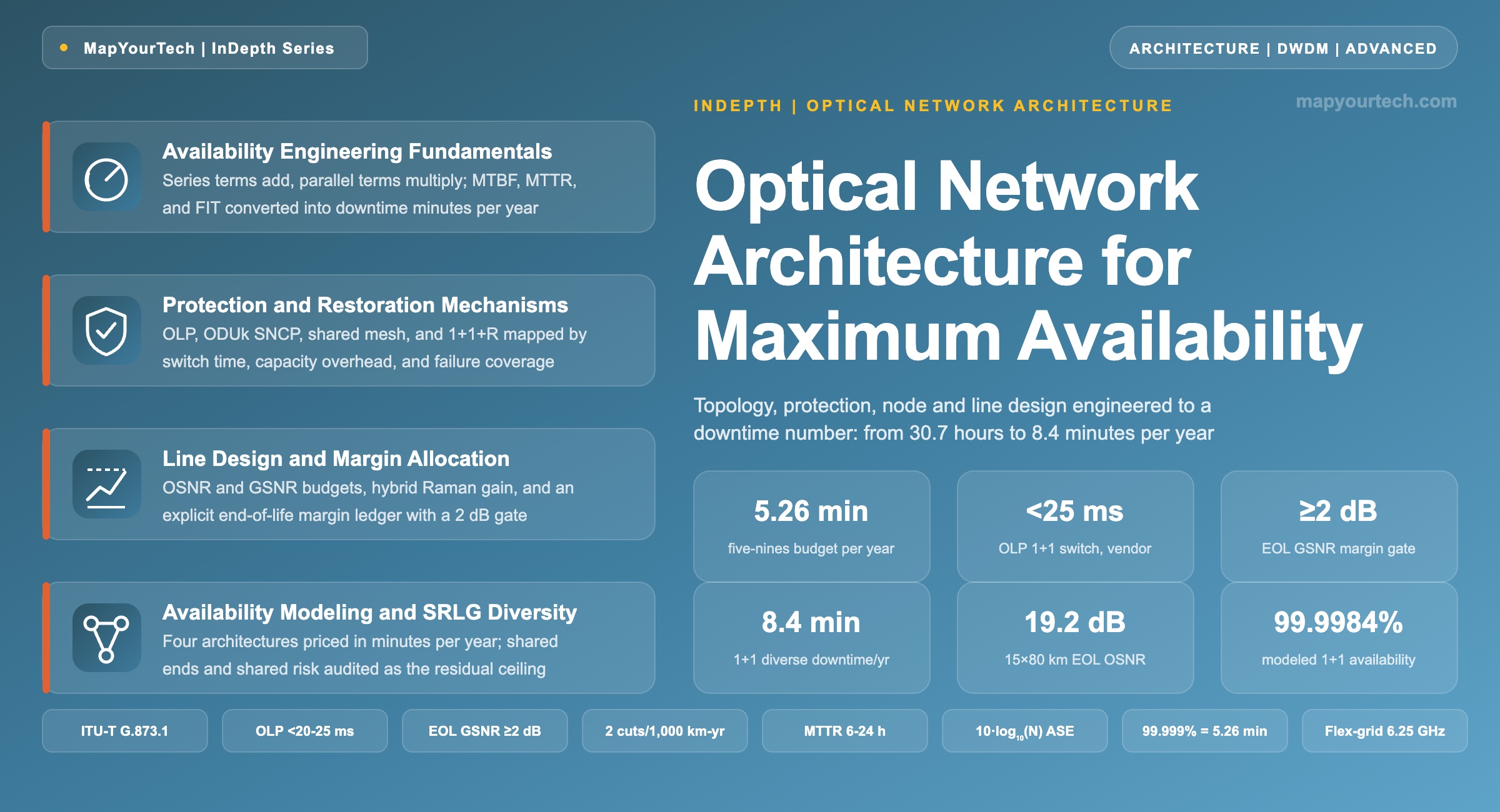
Optical Network Architecture Design for Maximum Availability
Availability is a design output, not an operational aspiration. This article works from measured failure statistics through topology selection, protection and restoration mechanisms, ROADM and line-system engineering, and closes with a worked model that prices each candidate architecture in minutes of downtime per year.
1. Introduction
A protection switch that completes in 23 ms and a fiber repair that takes 14 hours differ by a factor of two million, and an availability target decides which of the two a customer experiences. An unprotected 1,200 km wavelength on buried long-haul fiber accumulates roughly 31 hours of expected downtime per year from fiber cuts and equipment failures under typical planning assumptions; the same wavelength carried over two diverse routes with 1+1 protection accumulates minutes. The gap between those two numbers is not purchased with better components. It is purchased with architecture: the topology, the protection scheme, the node design, the optical margin, and the physical route diversity chosen before the first shelf is installed.
This article treats availability as a quantity to be engineered rather than a percentage to be promised. It defines the reliability arithmetic that converts component failure rates into service downtime, surveys the failure modes that dominate deployed networks, and then works through each architectural layer in turn: topology, protection and restoration mechanisms standardized in the ITU-T G.808 and G.873 series, reconfigurable optical add/drop multiplexer (ROADM) node structures, amplifier and margin engineering on the line, and the coherent transmission layer. The terminology around this subject is frequently blurred, so the distinctions between resiliency, redundancy, protection, survivability, and reliability in optical networks are worth fixing before the design work starts: protection is a pre-provisioned switch to dedicated or shared capacity, restoration is a computed re-route after failure, and availability is the fraction of time the service meets its specification.
The closing sections assemble these layers into a decision framework and apply it: a worked availability model compares unprotected, 1+1 protected, and shared-mesh restored variants of one long-haul service, and a service-mapping section matches architecture recipes to hyperscaler data center interconnect, national backbone, mobile transport, financial trading, and submarine use cases. Where the industry is moving in 2026 — multi-band line systems, hollow-core fiber, multi-rail transponders, and space-division multiplexing — each direction is assessed for what it changes in the availability calculation, not only in the capacity one.
Numbers throughout carry their evidence class in the sentence that states them: standard-specified values cite the recommendation, measured values name their source class, vendor figures are labeled as vendor claims, and theoretical limits are labeled as such. Planning values that vary by operator are marked as typical. The distinction matters because an availability commitment inherits the weakest evidence behind any number in its derivation.
2. Availability Engineering Fundamentals
Availability, MTBF, and MTTR Definitions
Availability is the probability that a repairable system is operational at an arbitrary instant. For a single element characterized by a mean time between failures (MTBF) and a mean time to repair (MTTR), steady-state availability is A = MTBF / (MTBF + MTTR), and unavailability is its complement U = 1 − A. Component reliability is commonly quoted in FIT (failures in time), the number of failures per 109 device-hours, so FIT = 109 / MTBF with MTBF in hours. A transponder with a planning MTBF of 300,000 hours is a 3,333 FIT device; an in-line amplifier at 500,000 hours is 2,000 FIT. Both figures are typical planning values of the kind vendors publish in reliability predictions per Telcordia SR-332 methodology, not measured fleet statistics, and mature designs frequently outperform them in the field.
Two composition rules generate every availability model in this article. Elements in series — a chain where any single failure takes the service down — multiply their availabilities, so unavailabilities approximately add when each is small. Elements in parallel — where the service survives unless all fail together — multiply their unavailabilities, which is the entire mathematical case for protection: squaring a small number produces a much smaller one.
Availability Composition Relations
A = MTBF / (MTBF + MTTR)        U = 1 − A
Aseries = A1 × A2 × … × An          Useries ≈ Σ Uₖ  (small U)
Uparallel = U1 × U2  (independent paths)
A: availability, U: unavailability, MTBF and MTTR in consistent time units. The parallel rule assumes statistically independent failures; shared risk between the paths adds a term covered in Section 11.
Availability Class Downtime Budgets
Translating percentages into clock time is what makes targets negotiable. Five nines (99.999%) allows 5.26 minutes of downtime per year — less than half of one fiber-cut repair — which is why five-nines services are never built on single unprotected paths. The table and chart below give the standard conversion; the logarithmic vertical axis on the chart is the honest way to show a range that spans four orders of magnitude.
| Class | Availability | Downtime per Year | Typical Service Tier |
|---|---|---|---|
| Two nines | 99% | 3.65 days | Best-effort, single access tail |
| Three nines | 99.9% | 8.76 h | Standard business connectivity |
| Four nines | 99.99% | 52.6 min | Enterprise WAN, protected wavelength |
| Five nines | 99.999% | 5.26 min | Carrier core, financial, mobile backhaul SLA |
| Six nines | 99.9999% | 31.5 s | Composite targets on fully diverse 1+1 paths |
Chart 1 data table
| Availability | Downtime (min/year) |
|---|---|
| 99% | 5,256 |
| 99.9% | 525.6 |
| 99.99% | 52.6 |
| 99.999% | 5.26 |
| 99.9999% | 0.53 |
Series Composition Across Network Segments
End-to-end services rarely live inside one administrative segment, and the series rule punishes concatenation. Access tails, metro rings, and long-haul cores each contribute their unavailability to the sum, so an end-to-end target must be decomposed into per-segment budgets before any segment is designed. The decomposition is a design decision with cost consequences: giving the long-haul segment a looser budget because its repairs are slow means the metro segments must be engineered tighter than their traffic alone would justify.
Practical Example — series budget across three segments
A service crosses two metro segments engineered to 99.99% each and one long-haul segment engineered to 99.999%. End-to-end availability is 0.9999 × 0.99999 × 0.9999 = 0.99979, which is 99.979% — approximately 110 minutes of expected downtime per year. Both metro segments together consume 20 times the downtime of the long-haul core. A customer who reads "five-nines core" in a proposal and expects five-nines service has been sold the wrong number: only the full series product is a commitment, and here it does not even reach four nines.
Design rule: MTTR is an availability lever equal in weight to MTBF. Halving repair time halves unavailability exactly as doubling MTBF does, and for buried fiber — where MTBF is fixed by geography and backhoes — sparing depth, dispatch contracts, and fault sectionalization are frequently the cheapest nines available.
Takeaway: Availability arithmetic is three relations: A = MTBF/(MTBF+MTTR), series availabilities multiply, parallel unavailabilities multiply. Every architecture decision in the remaining sections is an attempt to move a term from the series column into the parallel column at acceptable cost.
3. Failure Modes in Deployed Optical Networks
Fiber Plant Failure Statistics
Fiber cuts dominate transport downtime, and the classical measured baseline comes from published analyses of United States carrier outage records: cable damage on the order of 4.39 incidents per 1,000 sheath-miles per year, with cut frequency around 13 per 1,000 route-miles per year in metro plant and roughly 3 per 1,000 route-miles per year on long-haul routes. Those figures are decades old as measurements, and modern conduit practice improves on them, but their structure still holds in planning: metro fiber fails several times more often per kilometer than long-haul fiber because it shares shallow rights-of-way with every other utility, and excavation remains the leading cause. The same body of analysis attributes roughly 70% of network failures to single-link events — the case protection is designed for — with the remainder split among node failures and multi-failure events that only diversity planning addresses.
Read the Full Analysis with Premium
The remaining 88% of this article — the design numbers, trade-offs and field guidance — is part of MapYourTech Premium, along with the full premium library, courses and professional tools.
You May Also Like

-
Premium
-
August 18, 2026
-
Free
-
August 18, 2026
-
Free
-
August 18, 2026