
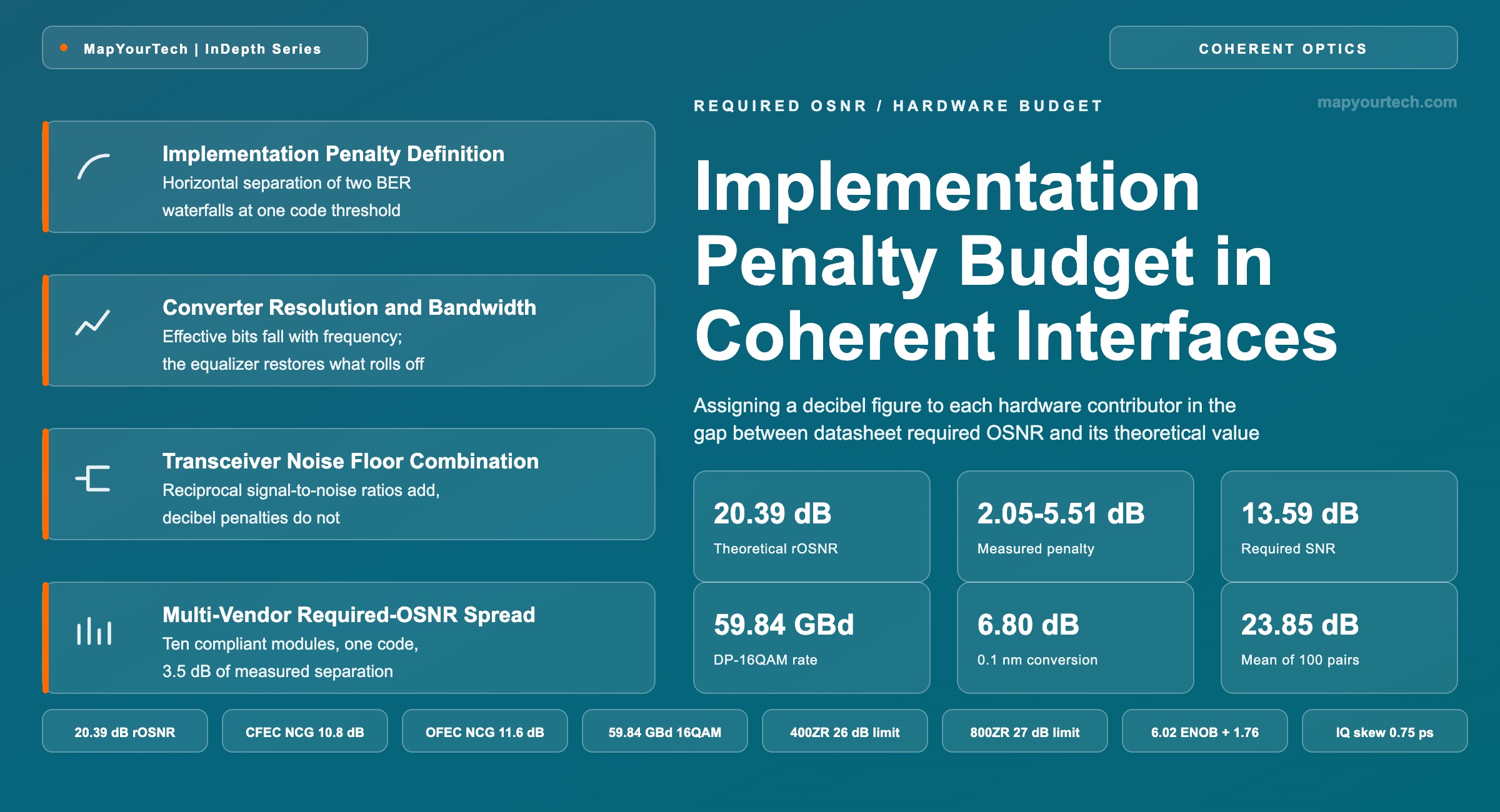
Implementation Penalty Budget in Coherent Interfaces
Required OSNR on a datasheet sits several decibels above the theoretical value for the same modulation and code. This article assigns a figure to each hardware contributor, shows how the contributors combine, and explains why the gap widens as symbol rate rises toward the front-end bandwidth limit.
Back-to-back performance is a floor, never a forecast.
What You Will Learn
- Define the implementation penalty as the horizontal separation of two BER waterfalls at one code threshold, using Figure 1 and the 20.39 dB theoretical reference derived in Section 2.
- Convert an electrical SNR to a 0.1 nm OSNR with the 6.80 dB reference term that applies at 59.84 GBd, and see the term rise to 9.76 dB at 118.203 GBd.
- Combine independent noise sources by adding reciprocal signal-to-noise ratios, and explain why nine contributors that would each cost under 0.4 dB alone together cost 2.14 dB.
- Quantify converter resolution through the 6.02 N + 1.76 dB relation, and read the 3.0 dB penalty that a 0.5 bit loss of effective resolution across the band produces.
- Anchor transmitter quality against the OIF 800ZR limits of 0.75 ps IQ skew, 5 degrees of quadrature error and 1 dB of IQ amplitude imbalance.
- Read the measured multi-vendor spread of 22.44 to 25.90 dB in Section 8 and convert it into a transceiver noise floor between 17.83 and 15.02 dB.
- Run the five-step extraction procedure of Figure 3 and state the seven conditions that make a penalty figure transferable between laboratories.
- Place the penalty correctly in a link budget alongside the 4.5 to 5.6 dB of specification headroom carried by the 400ZR and 800ZR agreements.
1. Introduction
Two 400 Gb/s pluggable modules built to the same Optical Internetworking Forum (OIF) agreement, running the same dual-polarization 16-state quadrature amplitude modulation (DP-16QAM) at the same 59.84 GBd and the same concatenated forward error correction (CFEC) code, differ by up to 3.5 dB in the optical signal-to-noise ratio (OSNR) they need to reach a post-FEC error-free state. That figure is not an estimate. At the OIF multi-vendor plugfests, ten QSFP-DD modules measured in loopback returned required OSNR values from 22.44 to 25.90 dB in a 0.1 nm reference bandwidth (measured, OIF plugfest campaign reported by Anritsu). Every one of those modules complies with the same agreement.
The theoretical value for that operating point is 20.39 dB. The separation between 20.39 dB and whatever a given module needs is the implementation penalty, and it is the single largest uncontrolled term an architect carries into a link budget. A planning tool that models fiber attenuation to a hundredth of a decibel per kilometre and amplifier noise figure to a tenth of a decibel commonly represents the entire transceiver as one scalar gap of about 3 dB. That scalar hides a hardware budget with named owners: converter resolution, front-end analog bandwidth against the symbol rate, modulator drive against Vπ, transmitter in-band noise, IQ skew and quadrature accuracy, laser phase noise against the carrier-recovery loop, and the noise the adaptive equalizer enhances while it flattens the channel.
Three groups of readers use that budget differently. A planner needs one number and its confidence interval, because the number sets reach. A procurement engineer needs the contributor list, because it explains why one supplier's module closes a span that another's does not at identical baud and identical code. A test engineer needs the measurement conditions, because a penalty figure quoted without its symbol rate, its code threshold, its receive power and its optical path is not comparable with anyone else's. This article serves all three: it defines the quantity, derives the theoretical reference, assigns a decibel figure to each contributor, shows the arithmetic that combines them, validates the result against published multi-vendor measurements, and states why the gap widens as symbol rate climbs toward the analog bandwidth of the front end.
Scope: the treatment covers back-to-back transceiver behaviour on point-to-point coherent interfaces in the 400 Gb/s to 1.6 Tb/s class, at the reference points defined by the OIF 400ZR and 800ZR agreements and the OpenZR+ Multi-Source Agreement (MSA). Line impairments accumulated over fiber spans, and the reach arithmetic they drive, are treated in the companion link-design walkthrough of the Shannon limit and in the line-rate threshold ladder, which quotes the implementation gap as a single model input.
2. Implementation Penalty Definition and Reference Conditions
The implementation penalty is the increase in required optical signal-to-noise ratio that a physical transceiver needs, relative to an ideal transceiver carrying the same constellation at the same symbol rate and reaching the same pre-forward-error-correction bit error rate. It is expressed in decibels, read at one fixed bit error rate, and referenced to the same 0.1 nm optical bandwidth on both sides. Nothing about the transmission line enters it.
Read the Full Analysis with Premium
The remaining 86% of this article — the design numbers, trade-offs and field guidance — is part of MapYourTech Premium, along with the full premium library, courses and professional tools.
You May Also Like

-
Free
-
September 4, 2026

-
Premium
-
September 4, 2026

-
Premium
-
September 4, 2026