Performance Monitoring Bin Semantics in Transport Networks
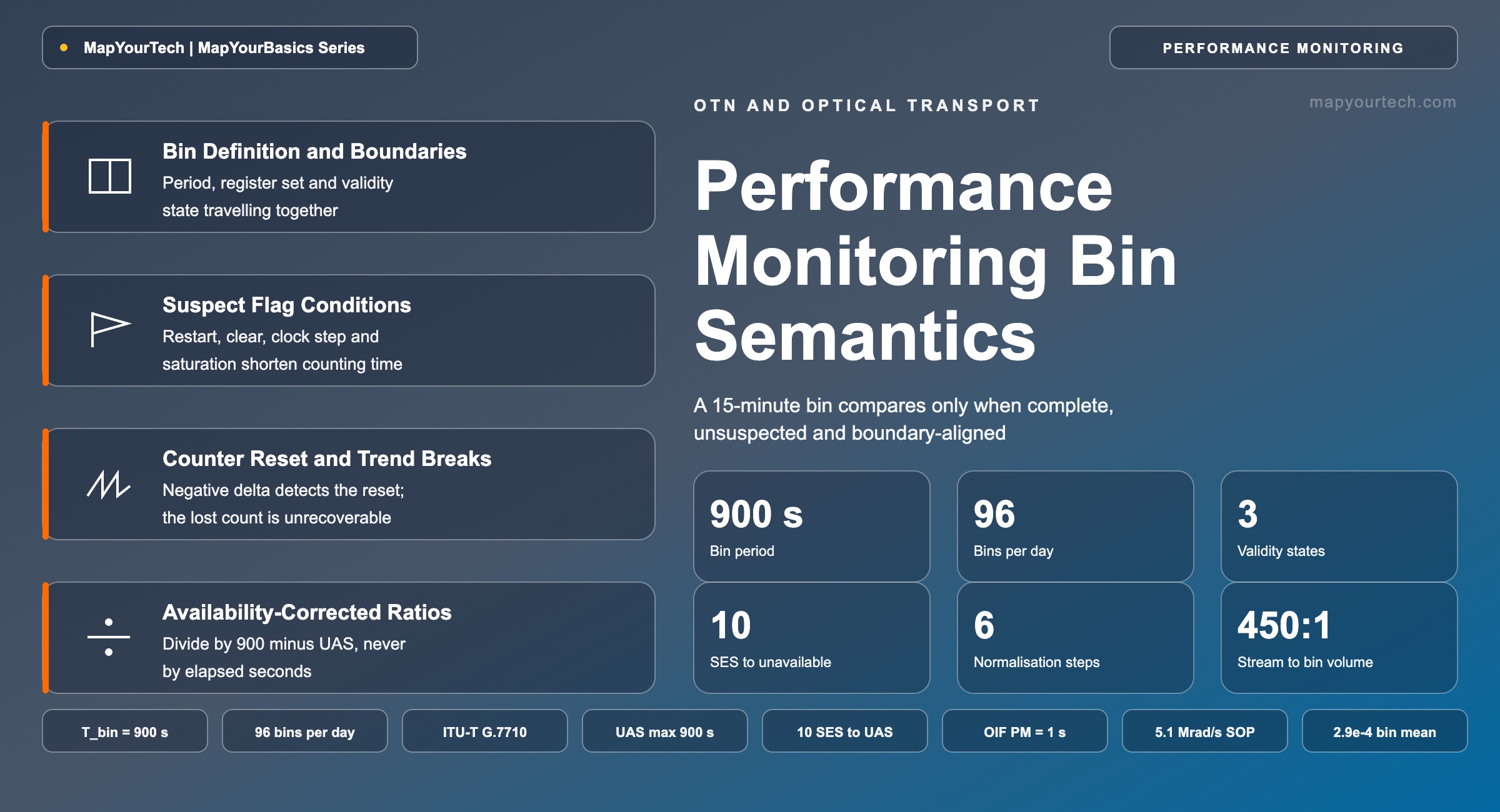
Two 15-minute registers compare only when both are complete, unsuspected and referenced to the same interval boundary, and a counter reset inside a bin changes what the number means without changing how it looks.
An alarm reports a defect; a trend reports a decision.
1. Introduction
A network management system that plots errored seconds against time is plotting a sequence of registers, not a sequence of measurements. Each register covers a fixed wall-clock period, resets at its boundary, and carries a state that says whether the equipment considers the contents trustworthy. ITU-T G.7710/Y.1701 specifies accumulation into 15-minute and 24-hour periods with threshold reporting on each (standard-specified), and every transport platform in service today implements that model at the device edge, whichever northbound interface sits above it.
The failure this article addresses is arithmetic performed across registers that do not describe the same thing. A bin interrupted by a card restart holds counts for part of its period. A bin whose counters were cleared by a maintenance action holds counts from after the clear only. A bin that went unavailable holds a denominator smaller than 900 seconds, because the error-performance model stops counting errored seconds once a path enters unavailable time. Subtracting one from another, ranking them, or feeding them to a regression treats all three as equivalent, and the resulting series contains structure that the network never produced.
The consequences reach past dashboards. Service level agreement verification uses these registers as the record of account. Threshold crossing alerts fire from them. Machine-learning models for predicting optical network failures are trained on them, and a model trained on unnormalised bins learns the shape of maintenance activity alongside the shape of degradation.
What follows fixes the vocabulary of a bin from first principles, states the arithmetic reason the 15-minute period was chosen and the reason it no longer covers every question asked of transport telemetry, enumerates the conditions that raise a suspect flag, traces what a counter reset does to a delta series, and gives the normalisation sequence to apply before any bin enters a time series. The scope is the transport layer — optical, OTN and Ethernet counters on line systems and transponders — and the treatment assumes familiarity with the error-performance parameters themselves.
2. Performance Monitoring Bin Definition and Interval Boundaries
A performance monitoring bin is a register set that accumulates the events of one monitored entity over a fixed wall-clock period, closes at the period boundary, and is stored with a validity state describing whether the accumulation ran uninterrupted. Counts are measured in events or seconds; the period is measured in seconds. The bin, not the individual second, is the unit that management interfaces expose.
2.1 Distinctions From Adjacent Quantities
Four neighbouring quantities get treated as interchangeable, and each conflation produces a different error. Bin period against collection period: the bin closes at the wall-clock boundary regardless of when the management system reads it, so a collector polling every 20 minutes still retrieves 15-minute bins and will silently skip one in three. Count against gauge: a count accumulates over the period and resets, while a gauge such as received optical power is sampled, so averaging counts and averaging gauges are different operations on different data. Elapsed seconds against available seconds: the period is always 900 seconds long, but the seconds in which the entity was counted as available can be fewer, and error ratios use the second figure. Suspect against zero: a suspect bin is an absence of information, while a zero bin is an assertion that nothing happened, and a collector that writes suspect bins as zero converts the first into the second.
T_bin = 900 s          N_bins_per_day = 86 400 / T_bin = 96
Available seconds in a bin:  T_avail = T_bin - UAS
Any error ratio in a bin: R = C / T_avail (not C / T_bin)- T_bin — accumulation period in seconds; 900 s for the 15-minute bin, 86 400 s for the 24-hour bin.
- UAS — unavailable seconds recorded inside the period; range 0–900 s.
- C — the count being normalised, in events or seconds.
- R — the resulting ratio, dimensionless when C is a second count.
Takeaway: A bin is a period, a register set and a validity state travelling together. Separating the number from the other two is what makes two bins look comparable when they are not.
3. Selection of the 15-Minute Accumulation Period
Nine hundred seconds was the shortest period that produced a countable number of errors at the line rates and error-ratio objectives of the synchronous era. At the STM-16 rate of 2.488 32 Gb/s, a 900-second period carries 2.24 × 1012 bits, so a path running at a bit error ratio of 1 × 10⁻¹² delivers about 2.2 errors into the register (computed). Shorten the period to 60 seconds and the same path delivers 0.15 expected errors, which reads as zero in almost every bin and as a spike in the occasional one. The period had to be long enough that the register content carried information rather than Poisson noise.
Three further properties made 900 seconds the working choice. It divides the hour and the day exactly, giving four bins per hour and 96 per day, so bins roll up into hourly and daily figures without remainder and align to the same wall-clock instants on every network element. It bounds the reporting latency of a threshold crossing alert to one period, which matched the response expectations of a staffed operations centre. And 96 registers per monitored parameter per day fits a fixed-size array in the limited non-volatile memory of a 1990s shelf controller, with the whole history retrievable over a management channel of a few hundred kb/s.
Chart 1: Expected Error Count per Accumulation Interval at a Bit Error Ratio of 1 × 10⁻¹². Logarithmic vertical scale. Values are the product of line rate, interval duration and error ratio (computed).
| Line rate | 1 s | 60 s | 900 s | 86 400 s |
|---|---|---|---|---|
| 2.488 Gb/s | 0.002 | 0.149 | 2.239 | 214.99 |
| 9.953 Gb/s | 0.010 | 0.597 | 8.958 | 859.96 |
| 400 Gb/s | 0.400 | 24.000 | 360.000 | 34560.00 |
The arithmetic that justified 900 seconds no longer holds at current line rates. One second at 400 Gb/s carries 4 × 1011 bits, as many as 161 seconds carried at the STM-16 rate (computed), so the statistical argument for a long period has been removed by capacity growth alone. Coherent lines make the point sharper still, because the parameter that carries advance warning is not a post-correction error count but the pre-FEC bit error ratio, which a receiver estimates continuously and which is already a rate rather than a rare event. Optical Internetworking Forum implementation agreements for the 400ZR and 800ZR interfaces define a programmable performance monitoring interval with a default of one second (standard-specified, OIF), so the module underneath a 15-minute register is frequently binning at 1 s and discarding the resolution on the way up.
Takeaway: The 15-minute period was a statistics and storage decision taken at 2.5 Gb/s. Both constraints have moved by more than two orders of magnitude, and the period has not.
4. Counter, Snapshot and Tidemark Measurement Methods
Three measurement methods share the same period and answer different questions. ITU-T G.7710/Y.1701 defines counter measurements, which accumulate event occurrences and reset at each boundary, and gauge measurements, which take the instantaneous value of a parameter and are reported as snapshots and as tidemarks (standard-specified). A snapshot is the value at one uniform instant inside the period, chosen so that snapshots taken across many network elements describe the same moment. A tidemark is the extreme value reached during the period, reported as a high tidemark and a low tidemark.
Method confusion produces two recurring defects. Comparing a snapshot against a tidemark treats one sample and one extreme as the same statistic, and on a parameter such as received optical power the two differ by whatever transient occurred in the period. Averaging tidemarks across bins produces a series with no physical referent at all, because the mean of a set of maxima is neither a maximum nor a mean. The OpenROADM device model exposes minimum, maximum and average variants as separate parameter names for exactly the binned optical quantities where this matters, including optical power input and output, optical signal-to-noise ratio, polarization dependent loss and chromatic dispersion (standard-specified, Open ROADM MSA).
| Method | What the register holds | Behaviour at boundary | Valid aggregation across bins |
|---|---|---|---|
| Count | Cumulative occurrences of an event in the period: ES, SES, BBE, UAS, protection switch count | Resets to zero | Sum, after availability correction |
| Snapshot | Instantaneous parameter value sampled at one uniform time in the period | Overwritten | Mean or median, as a sampled series |
| High tidemark | Highest value the parameter reached in the period | Re-armed | Maximum only |
| Low tidemark | Lowest value the parameter reached in the period | Re-armed | Minimum only |
4.1 Threshold Reporting Conditions
Threshold crossing alerts inherit the semantics of the register they watch. G.7710/Y.1701 defines a transient condition method, which treats each period separately and issues a threshold report as soon as the count reaches or crosses its threshold inside that period, and a standing condition method available for 15-minute periods, where the condition is raised at the crossing and cleared by a reset threshold report at the end of a period whose value has fallen to or below the reset threshold, provided no unavailable time occurred in that period (standard-specified). That proviso is the point of contact between threshold reporting and availability: a period containing unavailable time cannot clear a standing condition, so an alert can persist through a period whose count looks acceptable.
Thresholds themselves carry no standard values. Operators set them against their own objectives, which is why two networks carrying identical traffic can report different alert volumes from identical registers. The alarm and defect hierarchy underneath is standardised; the reporting layer above it is a local policy.
Takeaway: Counts, snapshots and tidemarks are three different measurements of the same period. Aggregating a tidemark as though it were a count or a snapshot is the most common silent error in a transport data pipeline.
5. Suspect Flag Generation Conditions
Equipment marks a bin suspect when the accumulation did not run cleanly for the whole period. The OpenROADM device model carries the state as a validity leaf with three values — complete, partial and suspect (standard-specified, Open ROADM MSA) — and the same three-way distinction appears under different names across vendor management interfaces and in the suspect interval flag of earlier ITU-T management models. The three states are not severity levels. Partial describes a period that is still open or that started late by design, such as the first bin after a service is provisioned. Suspect describes a period whose contents cannot be reconciled with its stated duration.
| Condition | Mechanism | Resulting state | Effect on the count |
|---|---|---|---|
| Controller or card restart | Register contents lost, accumulation restarts mid-period | Suspect | Covers part of the period only |
| Operator counter clear | Maintenance action zeroes the current register | Suspect | Covers time since the clear only |
| Time-of-day step | Clock correction moves the boundary; the period is longer or shorter than 900 s | Suspect | Denominator no longer 900 s |
| Monitoring enabled mid-period | PM was disabled on the entity when the period opened | Partial or suspect | Covers time since enablement |
| Service provisioned mid-period | Entity did not exist for the whole period | Partial | Covers time since creation |
| Current period read | Bin has not reached its boundary | Partial | Elapsed time less than 900 s |
| Facility placed out of service | Counting suspended by administrative state | Suspect | Gap with no accumulation |
| Register overflow | Count reaches the register maximum and saturates or wraps | Suspect | Underestimates the true count |
Two of these deserve separate attention because they are invisible in the count itself. A time-of-day step, whether from a network time protocol correction or a manual change, alters the length of the period without altering the register width, so a bin can hold 900 seconds of counting labelled as a shorter interval or the reverse. And a register that saturates reports a plausible ceiling value rather than an error, which reads as a stable measurement in a series and as an underestimate in an availability calculation.
Treat a missing validity field as suspect rather than as complete. Interfaces differ in whether they expose the state at all, and a collector that defaults an unknown state to complete converts every equipment restart in the network into a real dip in the error series.
Practical Example — a maintenance window that reads as an improvement
A line card is reseated at 14:07 during a planned window. The 14:00 to 14:15 bin restarts accumulation at 14:09 after the card completes its boot sequence, giving 360 seconds of counting inside a period labelled 900 seconds. The card had been reporting about 30 errored seconds per bin from a degrading connector. The bin closes with ES = 12 rather than 30, and the trend line falls by 60 percent at exactly the moment the fault was left untouched. The equipment marked the bin suspect. The collector wrote the number and dropped the flag.
Takeaway: Every condition that raises a suspect flag shortens the counting time without shortening the stated period, so a suspect bin always biases counts downward. An unfiltered suspect bin looks like good news.
6. Counter Reset Effects on Trend Continuity
Two counter models coexist on transport equipment, and a reset means something different in each. Binned registers reset at every boundary by design, so the value read from a closed bin is the count for that period and requires no differencing. Free-running counters, common on Ethernet and pluggable-module interfaces and on any parameter exposed through streaming telemetry, increase monotonically until something clears them, so the value for a period is the difference between two reads. A collector that mixes the two models — differencing a binned register, or summing a monotonic counter — produces a series that is wrong by construction long before any suspect flag is involved.
Detecting the reset is arithmetic; recovering the lost count is not. When consecutive reads give a decreasing value, the interval contains either a clear or a register wrap, and the two are distinguishable only if the register width is known and the wrap point can be predicted. The portion of the interval accumulated before the clear is gone in both cases, so the correct action is to mark the interval and exclude it, not to substitute the post-reset value. Writing the post-reset count as the interval delta understates the interval; writing the raw counter as the delta overstates every subsequent interval by the entire pre-reset history.
if  C(t2) >= C(t1):   delta = C(t2) - C(t1)          interval usable
if  C(t2) <  C(t1):   delta = undefined              interval suspect, exclude

Wrap case, only where register width W is known and documented:
delta = (W - C(t1)) + C(t2)- C(t1), C(t2) — counter values read at the start and end of the interval, in events.
- W — register modulus in events, typically 232 or 264.
- delta — count attributed to the interval, in events.
Takeaway: A reset is detectable from the delta sign and unrecoverable from the data. Exclude the interval, record the reason, and keep the gap visible in the series.
7. Availability Filtering and Bin Comparability
The error-performance model separates a path into available and unavailable time, and the counters behave differently in each. A path enters unavailable time at the onset of ten consecutive severely errored seconds, and those ten seconds belong to the unavailable period; it returns to available time at the onset of ten consecutive seconds that are not severely errored (standard-specified, ITU-T G.826 and G.8201). Errored seconds and severely errored seconds are counted in available time only, so the ten seconds that triggered the transition are reclassified out of the SES count and into the unavailable seconds count after the fact. The relationship between BBE, ES, SES and UAS is built on this reclassification, and it is retroactive by design.
Two consequences follow for bin comparability. First, the denominator changes: a bin holding 400 unavailable seconds has 500 available seconds, and an errored-second count of 20 is a ratio of 0.040 rather than 0.022. Second, a severe event reduces the SES count rather than increasing it once the path crosses into unavailability, so a bin containing a 12-minute outage can report fewer severely errored seconds than a bin containing a 12-second burst. Ranking bins by SES therefore ranks moderate impairment above total failure unless unavailable seconds are read alongside.
T_avail = 900 - UAS                       available seconds in the bin
ESR     = ES  / T_avail                   errored second ratio
SESR    = SES / T_avail                   severely errored second ratio
BBER    = BBE / (B_avail - B_ses)         background block error ratio

If T_avail = 0 the bin yields no ratio. Report unavailability, not a ratio of zero.- UAS — unavailable seconds in the bin, 0–900 s.
- ES, SES — errored and severely errored seconds counted in available time, in seconds.
- BBE — background block errors, that is errored blocks outside a severely errored second, in blocks.
- B_avail — total blocks in available time; B_ses — blocks contained in severely errored seconds.
Practical Example — two bins with the same errored-second count
Bin A on an ODU4 path records ES = 20, SES = 0, UAS = 0. Bin B on a parallel path records ES = 20, SES = 0, UAS = 400 following a protection event and its recovery. Read as counts, the two look identical. Corrected for availability, bin A gives an errored second ratio of 20 / 900 = 0.0222 and bin B gives 20 / 500 = 0.0400, which is 1.8 times higher on the same nominal count. A service-level report that sums errored seconds across a month and divides by the month treats both paths as equal and under-reports the second by the same factor.
Takeaway: Unavailable seconds are a denominator correction, not another error count. A bin without its unavailable-second value cannot yield a ratio at all.
8. Normalisation Procedure for Time-Series Ingestion
Six operations convert a raw bin into a record that can be compared with another record. The order is fixed, because each step depends on the one before it: a completeness test computed before the availability correction uses the wrong denominator, and a discontinuity check run after aggregation cannot see the reset that produced the aggregate.
Scaling a partial bin by the inverse of its completeness ratio is a defensible correction only within a narrow band. A bin that counted for 810 of 900 seconds and is scaled by 1.111 assumes the missing 90 seconds resembled the 810 that were measured, which holds for background error processes and fails for the burst that the restart may itself have caused. Below a completeness ratio of about 0.9 the assumption stops being defensible, and the bin belongs in the rejected store with its reason code rather than in the series with a correction factor.
Rejected bins are data. A month of rejected bins keyed by reason code shows which network elements restart most often, which maintenance procedures clear counters without recording it, and which entities never had monitoring enabled at all. The monitoring implementation checklist treats an empty counter and a disabled counter as separate findings for the same reason.
Takeaway: Normalisation is six ordered steps, and the output record carries four fields, not one: value, unit, denominator and validity. A pipeline that stores only the value has already lost the ability to compare.
9. Faster Polling and Streaming Telemetry Requirements
Events that determine service outcomes now complete inside a fraction of one bin. Field measurements on optical ground wire correlated state-of-polarization transients of up to 5.1 Mrad/s with documented lightning strikes (measured, Optics Express), and a coherent receiver either tracks that rotation or loses lock inside a few milliseconds. Protection switching completes within a 50 ms objective in ring specifications (standard-specified, ITU-T G.841). A pre-FEC bit error ratio excursion lasting 90 seconds carries the diagnosis of a marginal amplifier. Each of these is a sub-bin event, and a 15-minute register reports its average.
Chart 2: Transient Visibility Versus Aggregation Interval. A 90-second pre-FEC bit error ratio excursion from a 1 × 10⁻⁴ baseline to 2 × 10⁻³, shown at 1-second resolution, averaged into 60-second bins and averaged into 900-second bins (computed).
| Time from start | 1 s resolution | 60 s bins | 900 s bins |
|---|---|---|---|
| 0 s to 600 s | 1.00e-4 | 1.00e-4 | 2.90e-4 |
| 600 s to 660 s | 2.00e-3 | 2.00e-3 | 2.90e-4 |
| 660 s to 690 s | 2.00e-3 | 1.05e-3 | 2.90e-4 |
| 690 s to 900 s | 1.00e-4 | 1.05e-3 | 2.90e-4 |
| 900 s to 1800 s | 1.00e-4 | 1.00e-4 | 1.00e-4 |
The arithmetic sets the loss precisely. Ninety seconds at 2 × 10⁻³ inside 810 seconds at 1 × 10⁻⁴ averages to 2.9 × 10⁻⁴ across the bin (computed), so the true peak of twenty times baseline arrives at the management system as a bump of just under three times baseline. A threshold set to catch a twenty-fold excursion never fires. A threshold set low enough to catch a three-fold bin average fires on ordinary variation across the rest of the network.
9.1 Subscription in Place of Polling
Streaming telemetry inverts the collection model. The gRPC Network Management Interface defined by OpenConfig carries a Subscribe remote procedure call with three modes: SAMPLE, which pushes a value at a configured interval, ON_CHANGE, which pushes only when the value changes, and TARGET_DEFINED, which lets the device select the cadence for each leaf (standard-specified, OpenConfig gNMI specification). Devices commonly support one-second sample intervals on optical and interface parameters, with the achievable rate depending on the platform (vendor claim). In the IETF stack, RFC 8639 and RFC 8641 define subscription to notifications and to datastore updates, and work in the CCAMP area proposes a YANG data model that carries the G.7710 counts, snapshots and tidemarks over that push mechanism (proposed, IETF individual draft). The dashboard and collection architecture for these sources places gNMI subscriptions, NETCONF registers and controller-level streaming in one pipeline.
Faster collection does not retire the bin, and treating it as a replacement introduces a different error. Binned registers remain the record of account for service level verification, because they are the artefact the equipment itself computes, stores and can reproduce after the fact, and because the availability model that governs errored-second counting is defined on them. Streams carry diagnosis: the shape of a transient, the velocity of a drift, the correlation between a polarization event and a burst of corrected errors. A monitoring design that keeps both, and joins them on the interval boundary, answers the compliance question and the engineering question from the same collection path.
| Property | 15-minute binned register | Streaming subscription |
|---|---|---|
| Resolution | 900 s | 1 s or finer, platform dependent |
| Transport | NETCONF, TL1 or SNMP, pulled | gRPC or NETCONF notification, pushed |
| Loss behaviour | Bin survives on the device and can be re-read | Missed updates are gone unless replayed |
| Validity signalling | Explicit validity state per bin | Sequence numbers and timestamps per update |
| Availability model | Errored seconds filtered by availability | Raw values; availability computed downstream |
| Primary use | Service level verification and threshold reporting | Diagnosis, trend velocity and correlation |
Takeaway: A 900-second average removes the amplitude of any event shorter than the bin. Keep the bin as the compliance record and add a subscription for the events the bin was never able to describe.
10. Collector Design and Troubleshooting Reference
Storage volume separates the two collection paths by roughly two orders of magnitude. A network of 2 000 monitored entities with eight binned counters each produces 2 000 × 8 × 96 = 1 536 000 records per day. The same 2 000 entities streaming four parameters at a one-second interval produce 8 000 points per second, or 691 200 000 points per day, about 450 times the binned volume (computed). That ratio drives the usual arrangement: bins retained for the full service level agreement period, streams retained at full resolution for days and downsampled beyond that, with the raw window long enough to cover the time between an event and its investigation.
Retrieval mechanics matter as much as volume. The Open ROADM device model provides a historical bin retrieval that takes a bin-number range and a period type, and exposes the maximum number of stored bins the device supports for each period so a collector can size its polling loop against the equipment rather than against an assumption (standard-specified, Open ROADM MSA). A collector that polls less often than the history depth loses bins permanently; a collector that polls more often than the boundary period retrieves the same closed bin repeatedly and must deduplicate on the interval end time.
| Observation | Probable cause | Check |
|---|---|---|
| Counts fall to zero across many entities at once | Shelf controller restart clearing current registers | Validity state on the affected bins and the equipment event log |
| One bin in four missing from the series | Collector poll period longer than the bin period | Interval end timestamps for a uniform gap pattern |
| Errored seconds drop while an alarm is active | Path entered unavailable time; ES no longer counted | Unavailable seconds in the same bin |
| Delta series shows a large negative value | Free-running counter cleared or wrapped | Register width and any maintenance action recorded at that time |
| Counters permanently zero on a live service | Monitoring not enabled on the provisioned entity | Administrative state of the monitored entity |
| Bin length not equal to 900 s | Time-of-day correction inside the period | Clock synchronisation log against the interval boundary |
| Threshold alert persists on a clean bin | Standing condition cannot clear in a period containing unavailable time | Unavailable seconds in the period that should have cleared it |
Vendor behaviour varies within the standard. Transport platforms from Ciena, Nokia, Cisco, Adtran, Ribbon, ZTE and Huawei all implement 15-minute and 24-hour accumulation, and all expose a validity or suspect indication, but the field name, the enumeration values and the set of conditions that trigger it differ enough that a multi-vendor collector needs a per-platform mapping rather than a shared assumption. The service assurance model places that mapping in the mediation function, where normalisation belongs, rather than in the reporting layer where it would have to be repeated for every report.
Practical Example — reconciling a monthly availability figure
A monthly availability report for a 400G service shows 99.987 percent, and the customer disputes it against their own measurement of 99.971 percent. Reconciliation starts with bin arithmetic. The month holds 2 880 bins per entity. The collector stored 2 863, and 17 bins carry a suspect state from two controller restarts. Written as zero, those 17 bins contributed 15 300 seconds of implied availability that was never measured. Excluding them and reporting against 2 863 bins gives a figure inside the customer's measurement uncertainty, and the difference between the two numbers turns out to be the maintenance history rather than the network.
Takeaway: Size the collector against the device's stated history depth, deduplicate on interval end time, and keep the per-vendor validity mapping in the mediation layer.
11. Future Outlook
Two directions in current standards work change what a bin has to carry. Mapping the G.7710 measurement methods onto YANG push subscriptions makes the period a subscription parameter rather than a fixed property of the register, which turns the 15-minute bin into one configuration among several and raises the question of what validity means when a client selects its own period. Controller northbound interfaces are converging alarm and performance structures so that a streamed value and a stored bin describe the same entity through the same identifiers, which is the precondition for joining the two series at all.
The engineering skill that follows is less about the interval and more about provenance. A measurement pipeline that carries value, unit, denominator and validity end to end can absorb a change of period without changing any downstream calculation, because every consumer already knows what it is dividing by. A pipeline that carries only values will need the same repair work again at every resolution change, and it will keep producing series whose structure belongs to the collection process rather than to the network. Building the four-field record now is the part of this that does not expire.
12. Summary
A performance monitoring bin is a period, a register set and a validity state, and comparability requires all three. The 900-second period was chosen when 900 seconds at 2.5 Gb/s was the shortest interval that produced a countable number of errors at a bit error ratio of 1 × 10⁻¹², and one second at 400 Gb/s now carries more bits than 160 seconds did then. Suspect flags arise from restarts, counter clears, clock steps, mid-period enablement and register saturation, and every one of them shortens the counting time without shortening the stated period, so an unfiltered suspect bin biases a series downward. A counter reset is detectable from the sign of the delta and unrecoverable from the data, which makes exclusion with a reason code the only correct handling. Unavailable seconds are a denominator correction, and a bin with 400 unavailable seconds and 20 errored seconds carries a ratio 1.8 times higher than the same count in a fully available bin. Normalisation is six ordered operations producing a four-field record. And the events that now determine service outcomes — polarization transients measured to 5.1 Mrad/s, 50 ms protection switches, 90-second error excursions — are shorter than the bin that reports them, which is the case for adding a subscription alongside the register rather than in place of it.
Glossary
| Term | Definition |
|---|---|
| Accumulation period | The fixed wall-clock duration over which a register counts, 900 s or 86 400 s. |
| Background Block Error (BBE) | An errored block occurring outside a severely errored second. |
| Bin | One register set for one monitored entity over one accumulation period, stored with its validity state. |
| Errored Second (ES) | A one-second period containing at least one errored block or a defect, counted in available time. |
| Gauge measurement | An instantaneous parameter value, reported as a snapshot or as a tidemark. |
| Interval boundary | The wall-clock instant that closes one bin and opens the next. |
| Severely Errored Second (SES) | A one-second period in which the errored block count exceeds the defined proportion or a defect is present. |
| Snapshot | The parameter value sampled at one uniform time inside the period. |
| Suspect state | A validity value indicating the accumulation did not run for the whole stated period. |
| Threshold Crossing Alert (TCA) | A report issued when a monitored count reaches or crosses its configured threshold. |
| Tidemark | The highest or lowest value a parameter reached during the period. |
| Unavailable Second (UAS) | A second within an unavailable period, beginning at the onset of ten consecutive severely errored seconds. |
Further background on the defect and anomaly hierarchy that feeds these counters is covered in the maintenance and performance event model, and the downstream signalling behaviour in defect propagation and alarm indication mechanisms.
References
- ITU-T G.7710/Y.1701 — Common Equipment Management Function Requirements, ITU-T Study Group 15.
- ITU-T G.8201 — Error Performance Parameters and Objectives for Multi-Operator International Paths within Optical Transport Networks, ITU-T Study Group 15.
- ITU-T G.826 — End-to-End Error Performance Parameters and Objectives for International, Constant Bit-Rate Digital Paths and Connections, ITU-T Study Group 15.
- ITU-T G.841 — Types and Characteristics of SDH Network Protection Architectures, ITU-T Study Group 15.
- Open ROADM MSA — org-openroadm-pm-types and org-openroadm-device YANG Modules, Open ROADM MSA.
- IETF RFC 8641 — Subscription to YANG Notifications for Datastore Updates, Internet Engineering Task Force.
- OpenConfig — gNMI: gRPC Network Management Interface Specification, OpenConfig.
- Optical Internetworking Forum — Implementation Agreement for 800ZR, Optical Internetworking Forum.
- Charlton, Clarke, Doucet, O'Sullivan, Peterson, Wilson, Wellbrock and Bélanger — Field Measurements of SOP Transients in OPGW, with Time and Location Correlation to Lightning Strikes, Optics Express.
Related Articles on MapYourTech