
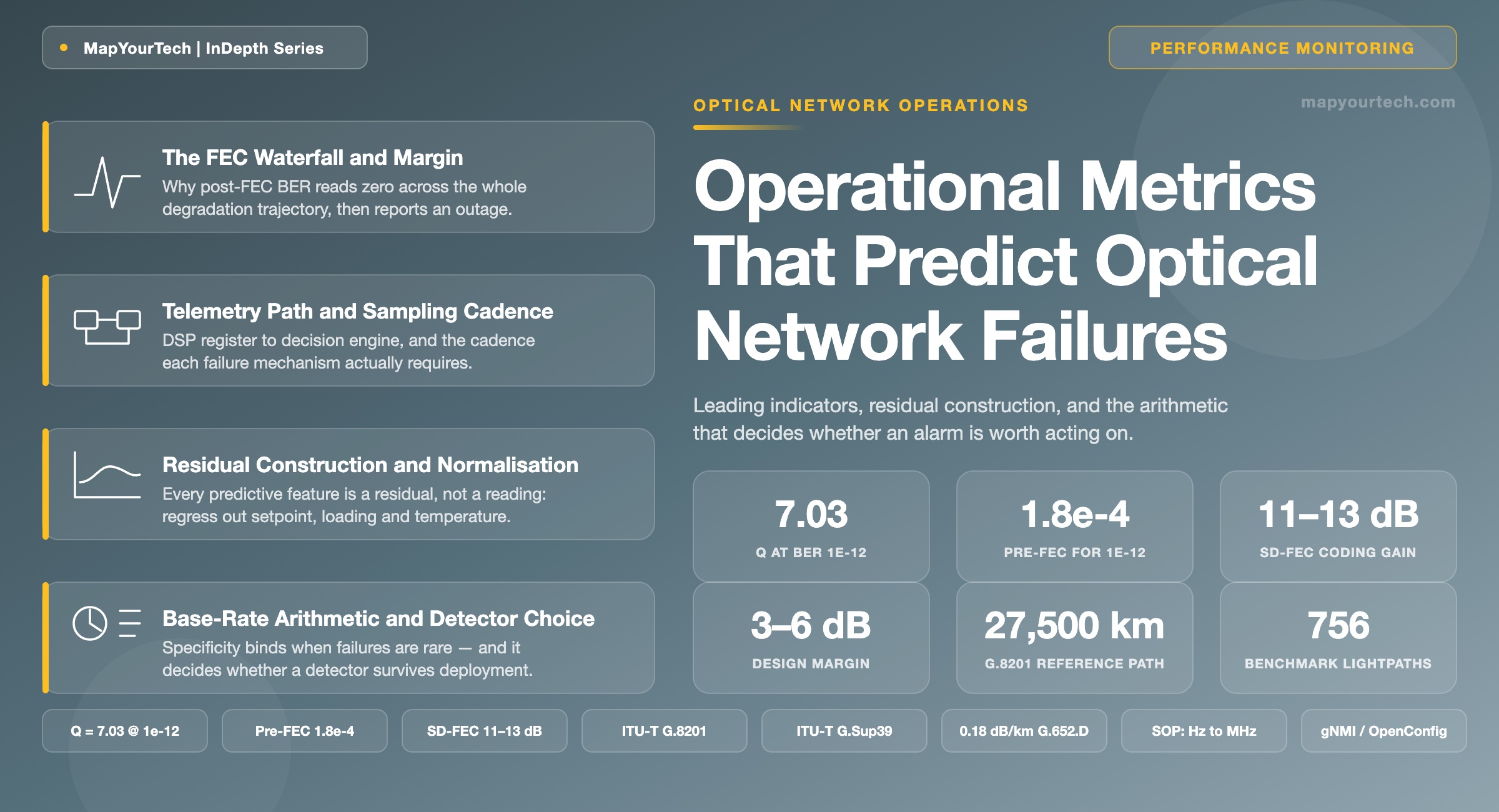
Operational Metrics That Predict Optical Network Failures
Which optical telemetry carries advance warning of a failure, which only records one after the fact, and how to tell the two apart before building a monitoring stack on the wrong signal.
1. Introduction
A coherent transponder reports post-forward-error-correction bit error ratio (post-FEC BER) as exactly zero for its entire service life, and then reports a traffic-affecting error burst. Nothing in that series told the operations team anything. The same transponder reports pre-FEC BER continuously, and that number moves through three orders of magnitude while the service stays error-free. One of those two counters is in almost every network management system dashboard. The other one is the only one of the pair that predicts anything.
This asymmetry is the subject of the article. Optical transport elements emit far more telemetry than any operations team consumes: per-channel optical power at every reconfigurable optical add-drop multiplexer (ROADM) degree, amplifier gain and pump bias current, laser bias and thermoelectric cooler current in every pluggable, chromatic dispersion and differential group delay estimates from every coherent digital signal processor (DSP), block error counts at every optical data unit (ODU) termination point, plus the alarm stream itself. The collection problem was solved once streaming telemetry over gRPC Network Management Interface (gNMI) displaced polling. The selection problem was not. Collecting a metric is easy; showing that its value at time t shifts the probability distribution of failure at time t + Δ is not.
The distinction that carries operational weight is between a metric that measures the state of a degradation process and a metric that measures the consequence of that process crossing a threshold. Amplified spontaneous emission accumulates, splice loss creeps, a pump laser's slope efficiency falls, a connector oxidises — all of these are slow, monotonic, and observable in the optical domain long before any digital counter increments. The digital counter increments when the accumulated penalty exceeds the receiver's correction capability. By construction, the counter is the last thing to move.
Optical transport networks still run predominantly on reactive fault management, which means service disruption is guaranteed at the onset of a soft failure rather than avoided (Scientific Reports, 2026). The industry response has been machine learning applied to telemetry, and the results are real: a Random Forest regressor with velocity, acceleration and rolling-statistic features predicted time-to-failure with 73.2 ± 0.03 s mean absolute error on a public optical telemetry benchmark of 756 lightpaths across four failure classes (Scientific Reports, 2026; measured on published benchmark data). But the model is downstream of the feature, and the feature is downstream of the metric. A gradient-boosted ensemble trained on link state and alarm counts will not outperform a straight line fitted to pre-FEC BER, because the information is not in the first pair of signals.
This article works through the physics of what degrades and how it becomes observable; the mathematics of margin, trend velocity and the base-rate arithmetic that determines whether an alarm is actionable; the architecture of a telemetry path that preserves the information rather than averaging it away; and the specific, named set of metrics that carry predictive content, alongside the equally specific set that does not. It is written for the engineer deciding what to subscribe to, at what cadence, and what to do with it.
Takeaway: Predictive value comes from metrics that track a continuous physical state variable with an operating margin above a threshold. Metrics that report the crossing of that threshold — post-FEC BER, loss-of-signal alarms, unavailable seconds — record failures rather than anticipate them, regardless of how frequently they are polled.
2. Foundational Concepts
2.1 Leading, Coincident and Lagging Indicators
Borrow the classification from reliability engineering and apply it strictly. A leading indicator changes measurably before the service-affecting event, with a lead time long enough to schedule an intervention. A coincident indicator changes at the same time as the event, which is useful for localisation and root cause but not for prevention. A lagging indicator changes only after the event, and its role is reporting and service-level accounting.
The test for a leading indicator is quantitative, not intuitive. For a candidate metric x and a failure event F at horizon Δ, the metric is leading if the conditional distribution of x given that F occurs within Δ separates from the distribution of x given that it does not — measured by area under the receiver operating characteristic curve, or by the precision achievable at an operationally acceptable recall. Many metrics that feel diagnostic fail this test because the separation exists but is far too small relative to the base rate of failure. Section 4.5 works the arithmetic.
2.2 Hard Failure and Soft Failure Definitions
A hard failure removes the signal: a fiber cut, a card power loss, a pump laser end-of-life open circuit. Transition time is milliseconds or less, the pre-event optical state is often normal, and the only available response is protection switching or restoration. Hard failures are not predictable from the signal that carries them, although they are sometimes predictable from a different observable — mechanical disturbance of a cable precedes a large fraction of aerial and duct fiber cuts, and that disturbance is visible in polarisation, not in power.
Soft failures are gradual degradations that shrink margin without removing service. An EDFA pump losing slope efficiency, a splice degrading under water ingress and freeze cycling, a wavelength-selective switch port with rising insertion loss, a transponder laser drifting in frequency, a connector accumulating contamination. Soft failures dominate the predictable population because they have a state trajectory, and a trajectory can be extrapolated.
The practical consequence is that a predictive monitoring programme should be scoped honestly. It will not predict the backhoe. It will predict the amplifier, the splice, the connector, the pluggable, and — through polarisation transients — a useful subset of the mechanical events that precede the backhoe by minutes to weeks.
2.3 Margin as the Observable State Variable
Every predictable optical failure reduces to one quantity: the difference between the signal quality delivered to the receiver and the signal quality the receiver needs. Everything else — pump current, span loss, tilt, contamination — is a mechanism that moves that difference. Design margin, typically 3–6 dB allocated at planning time for aging, temperature and component drift, is the budget the degradation process consumes.
This gives a single organising principle. The most predictive metric on any lightpath is the one closest to the margin itself, measured continuously, with the operating point held constant or explicitly divided out. Pre-FEC BER and the Q-factor derived from it sit closest, because the coherent DSP computes them from the actual received constellation after all impairments have been applied. Optical signal-to-noise ratio (OSNR) measured by an optical channel monitor sits one step further away, because it captures the linear noise contribution but not nonlinear interference; see the treatment of the OSNR-to-generalised-SNR gap in DWDM channel monitoring with OCM and OSA. Component-level metrics such as pump bias current sit furthest away but have the longest lead time, because they observe the mechanism directly rather than its integrated effect.
Build the metric hierarchy from the margin outward. Every metric earns its place by answering one of two questions: how much margin remains on this lightpath, or which component is consuming it. A metric that answers neither is inventory, not telemetry.
2.4 The FEC Waterfall and the Information Cliff
Forward error correction is the reason post-FEC BER carries no predictive information, and the mechanism is worth stating precisely. ITU-T G-series Supplement 39 states the relationship for the Reed-Solomon (255,239) code specified in ITU-T G.709: a bit error ratio of 1.8 × 10⁻⁴ at the FEC decoder input corresponds to 10-12 at the decoder output (standard-specified). Modern soft-decision FEC in coherent transponders operates with pre-FEC thresholds in the region of 2 × 10⁻², delivering net coding gain in the 11–13 dB range and post-FEC BER below 10-15 (typical values; exact threshold and gain vary by code and vendor implementation).
Read the Full Analysis with Premium
The remaining 89% of this article — the design numbers, trade-offs and field guidance — is part of MapYourTech Premium, along with the full premium library, courses and professional tools.
You May Also Like
-
Free
-
August 31, 2026
-
Free
-
August 27, 2026