
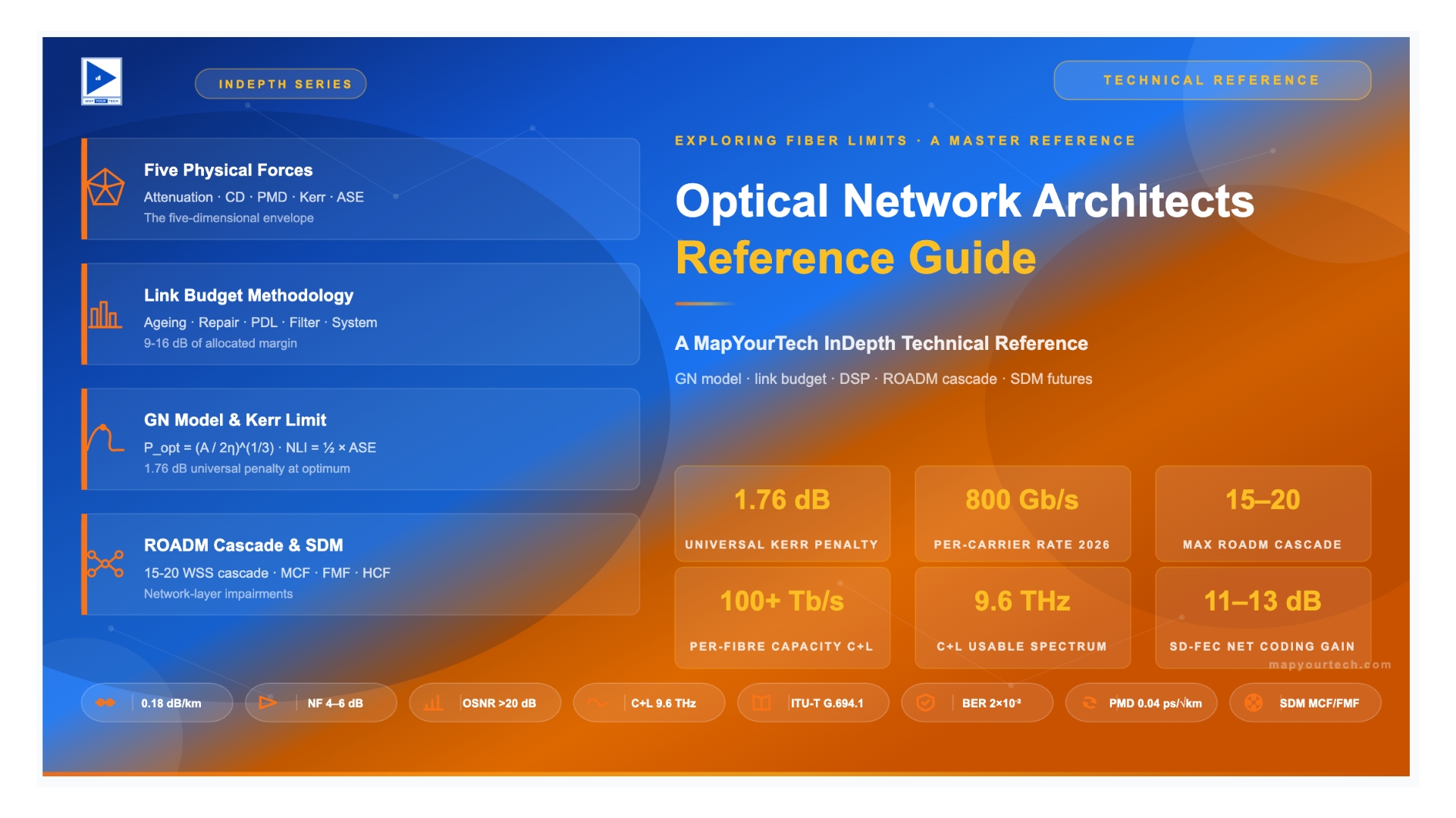
Optical Network Architects Reference Guide
Exploring fiber limits — the architect's working reference on every physical limit that bounds a coherent optical fibre link. From fibre physics and amplifier noise through dispersion, Kerr nonlinearity, Shannon, DSP, and FEC, to link-budget methodology, ROADM cascade, SDM impairments, and three worked case studies spanning metro to trans-Pacific.
Foundations and Theoretical Framework
1. Introduction
“Everything should be made as simple as possible, but not simpler.”
Every optical transmission engineer eventually confronts a question that sounds simple and proves deceptively hard: how fast can a single wavelength run on this fibre, and how far can it run? The answer is never a single number. It is a surface in a five-dimensional space whose axes are attenuation, chromatic dispersion, polarization-mode dispersion, nonlinearity, and noise. Push any axis too far and the link fails. Back off from one to buy margin on another and the economics of the deployment shift. This deep dive walks the full geometry of that space, explains the physics that gives it shape, and shows how each choice on a modern DWDM link — the fibre type, the span plan, the amplifier lineup, the modulation format, the symbol rate, the flex-grid allocation — is an instance of the same optimisation problem.
The headline figure in any optical-networking conference is line rate. In 2014 a commercial coherent wavelength carried 100 Gbps over transoceanic distances. As of 2026 a single wavelength carries 1.6 Tbps over metro spans and 1.2 Tbps transatlantic, and laboratory demonstrations have pushed beyond 3.2 Tbps per carrier. Those gains did not come from a single breakthrough. They came from incremental wins on every one of the five physical axes, compounded over a decade of DSP-assisted coherent receivers, wider spectrum, higher baud rates, denser constellations, stronger forward-error correction, and better fibre. Understanding how the gains compound requires understanding how the five limits interact, because the hardest part of the job is knowing which axis is binding on any given link.
A second motive for this series is practical. Field engineers, network architects, and product managers often inherit rules of thumb — "dispersion is no longer a problem in coherent systems", "PMD is only a legacy-fibre issue", "Shannon is the hard wall" — each of which is partly correct and dangerously incomplete. Chromatic dispersion is compensated in DSP, but its interaction with nonlinearity still bounds reach through the generalised Gaussian-noise model. Polarization-mode dispersion is small on new fibre, but high-baud-rate signals such as 200 Gbaud have a differential-group-delay tolerance that can be breached on legacy routes where nobody thought to look. Shannon sets a theoretical ceiling, but practical systems sit 3 to 6 dB below it even with soft-decision FEC because nonlinear interference is not additive Gaussian noise on a logarithmic power axis. Replacing rules of thumb with quantitative models is what separates a link that works from a link that surprises.
The third motive is forward-looking. The industry is running out of easy wins. Conventional single-mode fibre has a fundamental minimum attenuation near 0.14 dB/km set by Rayleigh scattering, and commercial G.654.E pure-silica-core fibre already operates at 0.155 to 0.17 dB/km over the C+L bands. The nonlinear Shannon limit, first articulated by Essiambre and refined by Poggiolini, bounds the achievable spectral efficiency on a given link at roughly 10 to 11 bit/s/Hz for long-haul distances. DSP power continues to grow, but the returns on the receiver side are diminishing. Future capacity will come from space — multi-core fibre, few-mode fibre, hollow-core fibre — and from better physical-layer orchestration. Understanding where today's limits come from is the only way to see where tomorrow's gains will come from.
Scope of this series. We treat a single DWDM channel on a standard single-mode fibre (SMF) link with coherent detection. We do not cover short-reach intra-datacentre pluggables (IM-DD, PAM4, 400G-DR4), submarine repeater electronic design in full detail, or space-division multiplexing beyond a brief future-directions treatment. Those topics extend the story but do not change the five physical limits examined here.
1.1 Map of the this Technical Reference
Throughout the articel we have first establishes the context, the historical arc, and the governing equations. Then works through attenuation, spans, and OSNR accumulation — the raw power budget. Next to covers the two linear dispersion effects, CD and PMD, that dominated the pre-coherent era and still bound modern high-baud-rate links on legacy fibre. Later its to treats the nonlinear Kerr effects (SPM, XPM, FWM), the scattering processes (SRS, SBS, GAWBS), and the Gaussian-noise model that ties them together. Next moves into spectral engineering — baud rate, Nyquist, modulation formats, the Shannon limit, the DSP chain, and forward-error correction. At end article closes with mixed-fiber hybrid links, three end-to-end case studies, a comparative analysis of the five limits, and a look at future directions.This article is developed based on author experience working on both end of the network ;i.e being a network user and as network design and engineering where extensive perspective is shared on what is needed in network being user and what are crucial information needed to design an Optical Network for scale.
2. Industry Context and Drivers
“The future is already here — it's just not evenly distributed.”
Understanding why fibre limits matter now, more than at any previous point in the 40-year history of optical telecommunications, requires situating the physics in the economic and traffic context that drives the industry. Traffic does not just grow; the shape of the demand changes, and that shape determines which physical limit becomes binding first.
2.1 The Shape of Modern Traffic
Global internet traffic grew at a compound rate near 30% through the 2010s, and although the rate has moderated as of 2026, three sectors are driving a new concentration of flows that changes how transmission engineers think about capacity. Hyperscale data-centre interconnect (DCI) has replaced long-haul voice and residential video as the dominant share of core-network fibre pairs. Artificial-intelligence training clusters now move exabytes of model parameters between data centres on dedicated wavelengths, often at the full 1.6 Tbps a single carrier can provide. Content-delivery networks push cached video toward the edge on shorter, denser regional routes. Each of these workloads has different reach-rate requirements, and each presses on a different physical limit.
Hyperscale DCI between sites separated by tens of kilometres is OSNR-rich and nonlinearity-limited: the signal does not need many amplifiers, so amplifier noise is small, but because the hyperscalers want to pack as much capacity into each fibre pair as possible, launch powers and channel counts run high enough that nonlinearity is the binding constraint. The AI training workload between data centres hundreds of kilometres apart is more symmetrical: it needs enough OSNR, and it needs enough PMD margin on whatever fibre the operator has available, which on legacy routes is often the issue. Transoceanic submarine systems are amplifier-noise-limited but also power-limited by the submarine electrical supply, and their design is essentially Shannon-bounded — every decibel of noise figure and every picometer of line-system ripple counts.
2.2 The 1.6T Line Rate Milestone
The 1.6 Tbps single-carrier wavelength became commercially available in 2024-2025 and entered mainstream deployment through 2026. The design lives at roughly 140-200 Gbaud depending on vendor, uses dual polarization, 64QAM or 128QAM with probabilistic constellation shaping, and a soft-decision FEC with roughly 20% overhead. It occupies 150-225 GHz of spectrum per channel on the ITU flex-grid, drops the reach relative to 800G at the same fibre by roughly a factor of two to three, and carries a price premium that falls every quarter as volume grows.
What is worth understanding is that the 1.6T generation pushes against every one of the five physical limits at once. The high constellation cardinality demands 25-26 dB of delivered OSNR for a modest margin on 20%-overhead FEC, which is 6-7 dB tighter than 800G 16QAM at the same baud rate. The 200 Gbaud symbol rate strains PMD tolerance on legacy fibre because the 5 picosecond symbol period is comparable to the differential group delay accumulated on older routes. The wide channel spacing increases the spectral tilt caused by Raman scattering across the full C+L band. The optimum launch power per channel is only 0.5-1 dB above 800G optima, but the GN-model nonlinear penalty is 2-3 dB worse at the same OSNR because the NLI noise scales quadratically with spectral density. Every one of these constraints is a reason 1.6T is the current state of the practicable art, and every one of them is a reason the next step to 3.2T requires new physics (space-division multiplexing, new fibre types, or analogue-coherent bandwidth beyond 300 GHz per channel).
2.3 Why Physical Limits Will Bite Harder, Not Softer
Through the 2000s and 2010s the industry absorbed traffic growth by stacking more channels into the C band, then into the L band, then by going coherent. Each of those moves gave roughly a decade of capacity growth per step. The decade ahead is different. The C+L fibre is near-full on main routes. Coherent modulation has captured the DSP gains available at CMOS-feasible clocks. Soft-decision FEC sits within 0.5 dB of Shannon. There is no obvious next step that yields a 10x capacity jump on existing fibre. The next 10x will require space — laying more fibre, activating multi-core or few-mode fibre, or accepting different economics for submarine cable builds that put 24-32 fibre pairs in the same ocean slot as earlier 4-8-pair designs. The physical limits examined in this series are therefore not curiosities; they are the binding constraints against which the next generation of optical network architecture will be evaluated.
3. Historical Evolution of Line Rate Scaling
“Those who cannot remember the past are condemned to repeat it.”
The story of line rate scaling is a story of successive dominant impairments. Each generation of system was limited by whichever physical effect first became binding, and each generation was defined by the technology that relieved that limit.
3.1 The 2.5 Gbps Era (late 1980s to mid-1990s)
At 2.5 Gbps direct-detection non-return-to-zero, chromatic dispersion was the hard wall. A G.652.B fibre at 1550 nm has D = 17 ps/nm/km. The 2.5 Gbps NRZ signal had a 3 dB optical bandwidth of 5 GHz, which is 0.04 nm at 1550 nm. The dispersion-limited reach is roughly (65,000 ps/nm)/(D), which places the CD limit at 3,800 km. In practice, residual OSNR and transmitter chirp reduced this to roughly 600-1,000 km without dispersion compensation. Regeneration every ~600 km was the standard design. The binding constraint was not Shannon, not attenuation, not PMD; it was the inability to run uncompensated dispersion beyond a few hundred kilometres.
3.2 The 10 Gbps Era (mid-1990s to mid-2000s)
10 Gbps NRZ narrowed the dispersion window by a factor of 16 (dispersion tolerance scales as 1/R_s^2). The practical dispersion limit without compensation became roughly 60 km, less than a single span. The industry responded by deploying dispersion-compensating fibre (DCF) modules between amplifiers, creating dispersion-managed links where the accumulated CD was zeroed every 100 km. This worked but traded a linear penalty (extra loss through the DCF) for a nonlinear penalty (the DCF has small effective area and high local nonlinearity). Dispersion-managed 10 Gbps links also exposed polarization-mode dispersion as the next binding constraint on legacy fibre.
3.3 The 40 Gbps Era and the Coherent Transition (mid-2000s to 2010)
40 Gbps NRZ had a dispersion tolerance of roughly 5 km, clearly impractical. The industry tried advanced direct-detection modulation formats — differential quaternary phase-shift keying (DQPSK), partial-response schemes, duobinary — each of which improved CD tolerance by 2 to 4 times and compressed the spectrum modestly. They were technically viable but never cost-competitive at high volume. The real transition was coherent detection, pioneered at 40 Gbps with dual-polarization QPSK, which moved all linear impairment compensation into the digital-signal-processor at the receiver and decoupled reach from chromatic dispersion entirely. Coherent at 40 Gbps was commercial by 2008 and displaced direct-detection at 40 Gbps by 2011.
3.4 The 100 Gbps Era (2010 to 2019)
Commercial coherent DP-QPSK at 100 Gbps, 32 Gbaud, was the reference line rate for most of the 2010s. It used 50 GHz channel spacing, soft-decision FEC with 20% overhead, and could reach 2,500-3,500 km on modern G.654 fibre or 1,500-2,500 km on G.652 fibre at OSNR margins of 2-3 dB. This is the generation that established the modern architecture: transponder DSP does all linear compensation, amplifier chain sets the OSNR floor, launch power sits at the GN-model optimum, and capacity per fibre scales primarily with the width of the usable spectrum.
3.5 The 200G to 800G Era (2019 to 2024)
Subsequent generations moved up the modulation and baud-rate ladder. 200 Gbps used DP-16QAM at 32 Gbaud or DP-QPSK at 64 Gbaud, the former for short reach and the latter for long. 400 Gbps DP-16QAM at 64 Gbaud became the workhorse metro/regional line rate around 2020-2022. 800 Gbps DP-64QAM at 96 Gbaud or DP-16QAM at 150 Gbaud filled the DCI and long-haul roles from 2022 onwards. Each generation used probabilistic constellation shaping to extract another 1 dB of spectral efficiency at the expense of slightly higher transponder DSP complexity.
3.6 The 1.6T Era and Beyond (2024 onwards)
1.6 Tbps per wavelength landed commercially in 2024-2025 on 140-200 Gbaud platforms with DP-64QAM or DP-128QAM and PCS. Line-rate reach at 1.6T is metro and short regional (300-800 km). Longer reach at the same line rate requires either multi-span dispersion management, distributed Raman to improve the amplifier chain, or a fall-back to 1.2T with lower constellation cardinality. Laboratory demonstrations in 2024 and 2025 have pushed per-carrier rates beyond 3.2 Tbps using extended-bandwidth DACs and ADCs at roughly 240 Gbaud, but commercial deployment remains two to four years out as of 2026.
| Era | Line rate | Dominant limit | Mitigation | Typical reach |
|---|---|---|---|---|
| 1988-1995 | 2.5 Gbps NRZ | Chromatic dispersion | Zero-dispersion fibre (G.653), regeneration | ~600 km |
| 1995-2005 | 10 Gbps NRZ | PMD on legacy fibre | Dispersion compensation modules, better fibre (G.652.D) | ~1,000 km |
| 2005-2010 | 40 Gbps NRZ → DQPSK | Dispersion and nonlinearity | Advanced modulation, early coherent (DP-QPSK) | ~600-1,500 km |
| 2010-2019 | 100 Gbps DP-QPSK | OSNR + nonlinearity | Coherent DSP, SD-FEC, C-band DWDM | ~2,500 km |
| 2019-2024 | 200G-800G, up to DP-64QAM | Nonlinear Shannon + baud rate | Higher baud, PCS, flex grid, C+L band | ~600-2,000 km |
| 2024 onwards | 1.6T DP-128QAM PCS | OSNR + PMD on legacy fibre | 200 Gbaud, G.654.E fibre, hybrid Raman | ~300-800 km |
4. The Five Forces at a Glance
“In theory, theory and practice are the same. In practice, they are not.”
Five physical effects set the ceiling on what an optical channel can carry over a fibre link. Each has its own scaling law, its own signature, and its own mitigation strategy, and they couple in ways that matter for every design decision. The subsequent parts of this series develop each in detail; this section gives the one-paragraph summary that lets a reader hold the whole picture in mind.
Attenuation is the exponential decay of optical power along the fibre, driven mainly by Rayleigh scattering at short wavelengths and infrared absorption at long wavelengths. It sets the span loss, which in turn sets the amplifier spacing and the accumulated OSNR. On G.652.D standard single-mode fibre near 1550 nm, attenuation is 0.19-0.22 dB/km. An 80 km span therefore loses about 16-18 dB. An EDFA with a 22 dB gain and a 5 dB noise figure can make up the loss, but each amplifier contributes noise. Twenty such spans accumulate roughly 18 dB of OSNR penalty relative to the transmitter.
Chromatic dispersion is the wavelength-dependence of the group velocity in the fibre. Near 1550 nm on G.652.D, dispersion is +17 ps/nm/km — a pulse at 1551 nm arrives 17 picoseconds later per kilometre than a pulse at 1550 nm. Because a modulated signal has finite spectral width, this stretches the symbol in time and, uncompensated, causes inter-symbol interference. In coherent systems the DSP corrects for several tens of thousands of ps/nm of accumulated dispersion with a finite-impulse-response equaliser, so chromatic dispersion on its own no longer limits reach directly. What it still does is interact with nonlinearity: in the presence of Kerr nonlinearity, the phase distortion from dispersion turns into amplitude distortion, and that is where most of the reach penalty on modern coherent links actually comes from.
Polarization-mode dispersion is the random differential delay between the two orthogonal polarization states of the fibre. Even a nominally circular single-mode fibre has residual birefringence from manufacturing tolerances, bends, twists, and thermal stress; the effect accumulates as a random walk along the length. The differential group delay (DGD) follows a Maxwellian distribution whose mean grows as the square root of length. For G.652.D, the PMD coefficient DPMD is specified at 0.04-0.10 ps/√km, giving ~0.4-1.0 picoseconds of DGD over 100 km. At 64 Gbaud this is a non-issue. At 200 Gbaud — the symbol period is 5 picoseconds — a legacy-fibre route with DPMD = 0.5 ps/√km over 400 km produces 10 ps of mean DGD, which is larger than the symbol period and exceeds any reasonable tolerance.
Kerr nonlinearity is the intensity-dependence of the fibre's refractive index. At high optical power the fibre core's index increases with the instantaneous field intensity, producing phase modulation proportional to power. This single physical effect manifests in three named forms: self-phase modulation (SPM), where a signal distorts its own phase; cross-phase modulation (XPM), where adjacent channels distort each other; and four-wave mixing (FWM), where three channels beat together to generate a fourth at a related frequency. On a WDM link, all three operate simultaneously and their combined impact on a coherent receiver is captured by the Gaussian-noise (GN) model as an equivalent additive-noise variance that scales as the cube of the launch power per channel. This cubic scaling is the reason an optical link has an optimum launch power: below it, the signal is lost in amplifier noise; above it, nonlinearity dominates.
OSNR, optical signal-to-noise ratio, is the quantity the modulation format ultimately competes against. OSNR accumulates through the link as a sum of inverse contributions: each amplifier contributes additive Gaussian noise, and the nonlinear noise contributes a further additive term through the GN model. The modulation format sets the required OSNR at the receiver — around 12-14 dB for dual-polarization QPSK with soft-decision FEC and 25% overhead, around 18-19 dB for 16QAM, around 24-25 dB for 64QAM — and the ratio of the link's delivered OSNR to the format's required OSNR is the system margin in dB. Double the bit count per symbol and you need roughly 6 dB more OSNR; that 6 dB has to be bought somewhere, which generally means halving the span count or halving the channel count.
Takeaway: Line rate does not scale freely with any single knob. Every factor of two in symbol rate costs 3 dB of OSNR, every factor of two in constellation cardinality costs roughly 6 dB, and every doubling of reach costs 3 dB. A modern 1.6T wavelength is the product of a decade of compound 1-2 dB improvements across all five physical axes — not a single breakthrough.
5. Theoretical Framework — the Nonlinear Schrödinger Equation
“The book of nature is written in the language of mathematics.”
The physics of a single-channel optical signal on a single-mode fibre is captured by one equation, the nonlinear Schrödinger equation (NLSE), and by its vector generalisation, the Manakov equation, for a dual-polarization signal. Every effect discussed in this series — attenuation, dispersion, nonlinearity — is a term in that equation. Before diving into each limit in isolation it helps to see them as coefficients of a single governing law.
Read the Full Analysis with Premium
The remaining 89% of this article — the design numbers, trade-offs and field guidance — is part of MapYourTech Premium, along with the full premium library, courses and professional tools.
You May Also Like

-
Free
-
September 4, 2026

-
Premium
-
September 4, 2026

-
Premium
-
September 4, 2026