Tag

Network performance

Browsing

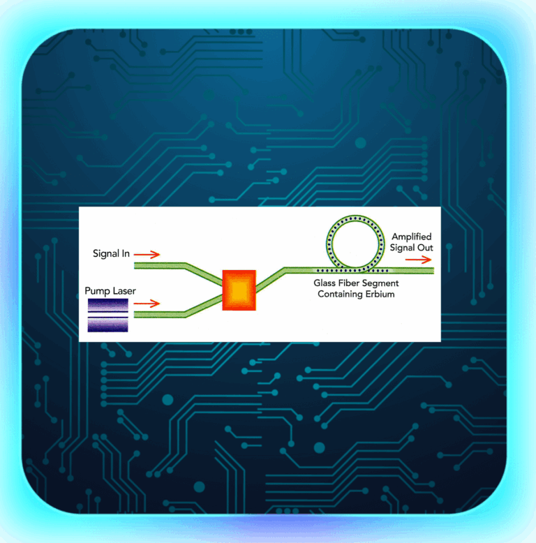
Optical Amplifiers (OAs) are key parts of today’s communication world. They help send data under the sea, land and even in space .In fact it is used in all electronic and telecommunications industry which has allowed human being develop and use gadgets and machines in daily routine.Due to OAs only; we are able to transmit data over a distance of few 100s too 1000s of kilometers.

Classification of OA Devices

Optical Amplifiers, integral in managing signal strength in fiber optics, are categorized based on their technology and application. These categories, as defined in ITU-T G.661, include Power Amplifiers (PAs), Pre-amplifiers, Line Amplifiers, OA Transmitter Subsystems (OATs), OA Receiver Subsystems (OARs), and Distributed Amplifiers.

amplifier

Scheme of insertion of an OA device

  1. Power Amplifiers (PAs): Positioned after the optical transmitter, PAs boost the signal power level. They are known for their high saturation power, making them ideal for strengthening outgoing signals.
  2. Pre-amplifiers: These are used before an optical receiver to enhance its sensitivity. Characterized by very low noise, they are crucial in improving signal reception.
  3. Line Amplifiers: Placed between passive fiber sections, Line Amplifiers are low noise OAs that extend the distance covered before signal regeneration is needed. They are particularly useful in point-multipoint connections in optical access networks.
  4. OA Transmitter Subsystems (OATs): An OAT integrates a power amplifier with an optical transmitter, resulting in a higher power transmitter.
  5. OA Receiver Subsystems (OARs): In OARs, a pre-amplifier is combined with an optical receiver, enhancing the receiver’s sensitivity.
  6. Distributed Amplifiers: These amplifiers, such as those using Raman pumping, provide amplification over an extended length of the optical fiber, distributing amplification across the transmission span.
Scheme of insertion of an OAT

Scheme of insertion of an OAT
Scheme of insertion of an OAR

Applications and Configurations

The application of these OA devices can vary. For instance, a Power Amplifier (PA) might include an optical filter to minimize noise or separate signals in multiwavelength applications. The configurations can range from simple setups like Tx + PA + Rx to more complex arrangements like Tx + BA + LA + PA + Rx, as illustrated in the various schematics provided in the IEC standards.

Building upon the foundational knowledge of Optical Amplifiers (OAs), it’s essential to understand the practical configurations of these devices in optical networks. According to the definitions of Booster Amplifiers (BAs), Pre-amplifiers (PAs), and Line Amplifiers (LAs), and referencing Figure 1 from the IEC standards, we can explore various OA device applications and their configurations. These setups illustrate how OAs are integrated into optical communication systems, each serving a unique purpose in enhancing signal integrity and network performance.

  1. Tx + BA + Rx Configuration: This setup involves a transmitter (Tx), followed by a Booster Amplifier (BA), and then a receiver (Rx). The BA is used right after the transmitter to increase the signal power before it enters the long stretch of the fiber. This configuration is particularly useful in long-haul communication systems where maintaining a strong signal over vast distances is crucial.
  2. Tx + PA + Rx Configuration: Here, the system comprises a transmitter, followed by a Pre-amplifier (PA), and then a receiver. The PA is positioned close to the receiver to improve its sensitivity and to amplify the weakened incoming signal. This setup is ideal for scenarios where the incoming signal strength is low, and enhanced detection is required.
  3. Tx + LA + Rx Configuration: In this configuration, a Line Amplifier (LA) is placed between the transmitter and receiver. The LA’s role is to amplify the signal partway through the transmission path, effectively extending the reach of the communication link. This setup is common in both long-haul and regional networks.
  4. Tx + BA + PA + Rx Configuration: This more complex setup involves both a BA and a PA, with the BA placed after the transmitter and the PA before the receiver. This combination allows for both an initial boost in signal strength and a final amplification to enhance receiver sensitivity, making it suitable for extremely long-distance transmissions or when signals pass through multiple network segments.
  5. Tx + BA + LA + Rx Configuration: Combining a BA and an LA provides a powerful solution for extended reach. The BA boosts the signal post-transmission, and the LA offers additional amplification along the transmission path. This configuration is particularly effective in long-haul networks with significant attenuation.
  6. Tx + LA + PA + Rx Configuration: Here, the LA is used for mid-path amplification, while the PA is employed near the receiver. This setup ensures that the signal is sufficiently amplified both during transmission and before reception, which is vital in networks with long spans and higher signal loss.
  7. Tx + BA + LA + PA + Rx Configuration: This comprehensive setup includes a BA, an LA, and a PA, offering a robust solution for maintaining signal integrity across very long distances and complex network architectures. The BA boosts the initial signal strength, the LA provides necessary mid-path amplification, and the PA ensures that the receiver can effectively detect the signal.

Characteristics of Optical Amplifiers

Each type of OA has specific characteristics that define its performance in different applications, whether single-channel or multichannel. These characteristics include input and output power ranges, wavelength bands, noise figures, reflectance, and maximum tolerable reflectance at input and output, among others.

For instance, in single-channel applications, a Power Amplifier’s characteristics would include an input power range, output power range, power wavelength band, and signal-spontaneous noise figure. In contrast, for multichannel applications, additional parameters like channel allocation, channel input and output power ranges, and channel signal-spontaneous noise figure become relevant.

Optically Amplified Transmitters and Receivers

In the realm of OA subsystems like OATs and OARs, the focus shifts to parameters like bit rate, application code, operating signal wavelength range, and output power range for transmitters, and sensitivity, overload, and bit error ratio for receivers. These parameters are critical in defining the performance and suitability of these subsystems for specific applications.

Understanding Through Practical Examples

To illustrate, consider a scenario in a long-distance fiber optic communication system. Here, a Line Amplifier might be employed to extend the transmission distance. This amplifier would need to have a low noise figure to minimize signal degradation and a high saturation output power to ensure the signal remains strong over long distances. The specific values for these parameters would depend on the system’s requirements, such as the total transmission distance and the number of channels being used.

Advanced Applications of Optical Amplifiers

  1. Long-Haul Communication: In long-haul fiber optic networks, Line Amplifiers (LAs) play a critical role. They are strategically placed at intervals to compensate for signal loss. For example, an LA with a high saturation output power of around +17 dBm and a low noise figure, typically less than 5 dB, can significantly extend the reach of the communication link without the need for electronic regeneration.
  2. Submarine Cables: Submarine communication cables, spanning thousands of kilometers, heavily rely on Distributed Amplifiers, like Raman amplifiers. These amplifiers uniquely boost the signal directly within the fiber, offering a more distributed amplification approach, which is crucial for such extensive undersea networks.
  3. Metropolitan Area Networks: In shorter, more congested networks like those in metropolitan areas, a combination of Booster Amplifiers (BAs) and Pre-amplifiers can be used. A BA, with an output power range of up to +23 dBm, can effectively launch a strong signal into the network, while a Pre-amplifier at the receiving end, with a very low noise figure (as low as 4 dB), enhances the receiver’s sensitivity to weak signals.
  4. Optical Add-Drop Multiplexers (OADMs): In systems using OADMs for channel multiplexing and demultiplexing, Line Amplifiers help in maintaining signal strength across the channels. The ability to handle multiple channels, each potentially with different power levels, is crucial. Here, the channel addition/removal (steady-state) gain response and transient gain response become significant parameters.

Technological Innovations and Challenges

The development of OA technologies is not without challenges. One of the primary concerns is managing the noise, especially in systems with multiple amplifiers. Each amplification stage adds some noise, quantified by the signal-spontaneous noise figure, which can accumulate and degrade the overall signal quality.

Another challenge is the management of Polarization Mode Dispersion (PMD) in Line Amplifiers. PMD can cause different light polarizations to travel at slightly different speeds, leading to signal distortion. Modern LAs are designed to minimize PMD, a critical parameter in high-speed networks.

Future of Optical Amplifiers in Industry

The future of OAs is closely tied to the advancements in fiber optic technology. As data demands continue to skyrocket, the need for more efficient, higher-capacity networks grows. Optical Amplifiers will continue to evolve, with research focusing on higher power outputs, broader wavelength ranges, and more sophisticated noise management techniques.

Innovations like hybrid amplification techniques, combining the benefits of Raman and Erbium-Doped Fiber Amplifiers (EDFAs), are on the horizon. These hybrid systems aim to provide higher performance, especially in terms of power efficiency and noise reduction.

References

ITU-T :https://www.itu.int/en/ITU-T/Pages/default.aspx

Image :https://www.chinacablesbuy.com/guide-to-optical-amplifier.html

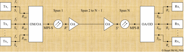
Optical networks are the backbone of the internet, carrying vast amounts of data over great distances at the speed of light. However, maintaining signal quality over long fiber runs is a challenge due to a phenomenon known as noise concatenation. Let’s delve into how amplified spontaneous emission (ASE) noise affects Optical Signal-to-Noise Ratio (OSNR) and the performance of optical amplifier chains.

The Challenge of ASE Noise

ASE noise is an inherent byproduct of optical amplification, generated by the spontaneous emission of photons within an optical amplifier. As an optical signal traverses through a chain of amplifiers, ASE noise accumulates, degrading the OSNR with each subsequent amplifier in the chain. This degradation is a crucial consideration in designing long-haul optical transmission systems.

Understanding OSNR

OSNR measures the ratio of signal power to ASE noise power and is a critical parameter for assessing the performance of optical amplifiers. A high OSNR indicates a clean signal with low noise levels, which is vital for ensuring data integrity.

Reference System for OSNR Estimation

As depicted in Figure below), a typical multichannel N span system includes a booster amplifier, N−1 line amplifiers, and a preamplifier. To simplify the estimation of OSNR at the receiver’s input, we make a few assumptions:

Representation of optical line system interfaces (a multichannel N-span system)
  • All optical amplifiers, including the booster and preamplifier, have the same noise figure.
  • The losses of all spans are equal, and thus, the gain of the line amplifiers compensates exactly for the loss.
  • The output powers of the booster and line amplifiers are identical.

Estimating OSNR in a Cascaded System

E1: Master Equation For OSNR

E1: Master Equation For OSNR

Pout is the output power (per channel) of the booster and line amplifiers in dBm, L is the span loss in dB (which is assumed to be equal to the gain of the line amplifiers), GBA is the gain of the optical booster amplifier in dB, NFis the signal-spontaneous noise figure of the optical amplifier in dB, h is Planck’s constant (in mJ·s to be consistent with Pout in dBm), ν is the optical frequency in Hz, νr is the reference bandwidth in Hz (corresponding to c/Br ), N–1 is the total number of line amplifiers.

The OSNR at the receivers can be approximated by considering the output power of the amplifiers, the span loss, the gain of the optical booster amplifier, and the noise figure of the amplifiers. Using constants such as Planck’s constant and the optical frequency, we can derive an equation that sums the ASE noise contributions from all N+1 amplifiers in the chain.

Simplifying the Equation

Under certain conditions, the OSNR equation can be simplified. If the booster amplifier’s gain is similar to that of the line amplifiers, or if the span loss greatly exceeds the booster gain, the equation can be modified to reflect these scenarios. These simplifications help network designers estimate OSNR without complex calculations.

1)          If the gain of the booster amplifier is approximately the same as that of the line amplifiers, i.e., GBA » L, above Equation E1 can be simplified to:

osnr_2

E1-1

2)          The ASE noise from the booster amplifier can be ignored only if the span loss L (resp. the gain of the line amplifier) is much greater than the booster gain GBA. In this case Equation E1-1 can be simplified to:

E1-2

3)          Equation E1-1 is also valid in the case of a single span with only a booster amplifier, e.g., short‑haul multichannel IrDI in Figure 5-5 of [ITU-T G.959.1], in which case it can be modified to:

E1-3

4)          In case of a single span with only a preamplifier, Equation E1 can be modified to:

Practical Implications for Network Design

Understanding the accumulation of ASE noise and its impact on OSNR is crucial for designing reliable optical networks. It informs decisions on amplifier placement, the necessity of signal regeneration, and the overall system architecture. For instance, in a system where the span loss is significantly high, the impact of the booster amplifier on ASE noise may be negligible, allowing for a different design approach.

Conclusion

Noise concatenation is a critical factor in the design and operation of optical networks. By accurately estimating and managing OSNR, network operators can ensure signal quality, minimize error rates, and extend the reach of their optical networks.

In a landscape where data demands are ever-increasing, mastering the intricacies of noise concatenation and OSNR is essential for anyone involved in the design and deployment of optical communication systems.

References

https://www.itu.int/rec/T-REC-G/e

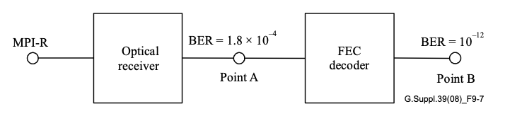
Forward Error Correction (FEC) has become an indispensable tool in modern optical communication, enhancing signal integrity and extending transmission distances. ITU-T recommendations, such as G.693, G.959.1, and G.698.1, define application codes for optical interfaces that incorporate FEC as specified in ITU-T G.709. In this blog, we discuss the significance of Bit Error Ratio (BER) in FEC-enabled applications and how it influences optical transmitter and receiver performance.

The Basics of FEC in Optical Communications

FEC is a method of error control for data transmission, where the sender adds redundant data to its messages. This allows the receiver to detect and correct errors without the need for retransmission. In the context of optical networks, FEC is particularly valuable because it can significantly lower the BER after decoding, thus ensuring the accuracy and reliability of data across vast distances.

BER Requirements in FEC-Enabled Applications

For certain optical transport unit rates (OTUk), the system BER is mandated to meet specific standards only after FEC correction has been applied. The optical parameters, in these scenarios, are designed to achieve a BER no worse than 10−12 at the FEC decoder’s output. This benchmark ensures that the data, once processed by the FEC decoder, maintains an extremely high level of accuracy, which is crucial for high-performance networks.

Practical Implications for Network Hardware

When it comes to testing and verifying the performance of optical hardware components intended for FEC-enabled applications, achieving a BER of 10−12 at the decoder’s output is often sufficient. Attempting to test components at 10−12 at the receiver output, prior to FEC decoding, can lead to unnecessarily stringent criteria that may not reflect the operational requirements of the application.

Adopting Appropriate BER Values for Testing

The selection of an appropriate BER for testing components depends on the specific application. Theoretical calculations suggest a BER of 1.8×10⁻⁴at the receiver output (Point A) to achieve a BER of 10−12 at the FEC decoder output (Point B). However, due to variations in error statistics, the average BER at Point A may need to be lower than the theoretical value to ensure the desired BER at Point B. In practice, a BER range of 10−5 to 10−6 is considered suitable for most applications.

Conservative Estimation for Receiver Sensitivity

By using a BER of 10−6 for component verification, the measurements of receiver sensitivity and optical path penalty at Point A will be conservative estimates of the values after FEC correction. This approach provides a practical and cost-effective method for ensuring component performance aligns with the rigorous demands of FEC-enabled systems.

Conclusion

FEC is a powerful mechanism that significantly improves the error tolerance of optical communication systems. By understanding and implementing appropriate BER testing methodologies, network operators can ensure their components are up to the task, ultimately leading to more reliable and efficient networks.

As the demands for data grow, the reliance on sophisticated FEC techniques will only increase, cementing BER as a fundamental metric in the design and evaluation of optical communication systems.

References

https://www.itu.int/rec/T-REC-G/e

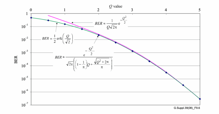
Signal integrity is the cornerstone of effective fiber optic communication. In this sphere, two metrics stand paramount: Bit Error Ratio (BER) and Q factor. These indicators help engineers assess the performance of optical networks and ensure the fidelity of data transmission. But what do these terms mean, and how are they calculated?

What is BER?

BER represents the fraction of bits that have errors relative to the total number of bits sent in a transmission. It’s a direct indicator of the health of a communication link. The lower the BER, the more accurate and reliable the system.

ITU-T Standards Define BER Objectives

The ITU-T has set forth recommendations such as G.691, G.692, and G.959.1, which outline design objectives for optical systems, aiming for a BER no worse than 10−12 at the end of a system’s life. This is a rigorous standard that guarantees high reliability, crucial for SDH and OTN applications.

Measuring BER

Measuring BER, especially as low as 10−12, can be daunting due to the sheer volume of bits required to be tested. For instance, to confirm with 95% confidence that a system meets a BER of 10−12, one would need to test 3×1012 bits without encountering an error — a process that could take a prohibitively long time at lower transmission rates.

The Q Factor

The Q factor measures the signal-to-noise ratio at the decision point in a receiver’s circuitry. A higher Q factor translates to better signal quality. For a BER of 10−12, a Q factor of approximately 7.03 is needed. The relationship between Q factor and BER, when the threshold is optimally set, is given by the following equations:

The general formula relating Q to BER is:

bertoq

A common approximation for high Q values is:

ber_t_q_2

For a more accurate calculation across the entire range of Q, the formula is:

ber_t_q_3

Practical Example: Calculating BER from Q Factor

Let’s consider a practical example. If a system’s Q factor is measured at 7, what would be the approximate BER?

Using the approximation formula, we plug in the Q factor:

This would give us an approximate BER that’s indicative of a highly reliable system. For exact calculations, one would integrate the Gaussian error function as described in the more detailed equations.

Graphical Representation

ber_t_q_4

The graph typically illustrates these relationships, providing a visual representation of how the BER changes as the Q factor increases. This allows engineers to quickly assess the signal quality without long, drawn-out error measurements.

Concluding Thoughts

Understanding and applying BER and Q factor calculations is crucial for designing and maintaining robust optical communication systems. These concepts are not just academic; they directly impact the efficiency and reliability of the networks that underpin our modern digital world.

References

https://www.itu.int/rec/T-REC-G/e

The ITU standards define a “suspect internal flag” which should indicate if the data contained within a register is ‘suspect’ (conditions defined in Q.822). This is more frequently referred to as the IDF (Invalid Data Flag).

PM is bounded by strict data collection  rules as defined in standards. When the collection of PM parameters is affected then  PM system labels the collection of data as suspect with an Invalid Data Flag (IDF). For the sake of identification; some unique flag  is shown next to corresponding counter.

The purpose of the flag is to indicate when the data in the PM bin may not be complete or may have been affected such that the data is not completely reliable. The IDF does not mean the software is contingent.

Some of the common reasons  for setting the IDF include:

  • a collection time period that does not start within +/- 1 second of the nominal collection window start time.
  • a time interval that is inaccurate by +/- 10 seconds (or more)
  • the current time period changes by +/- 10 seconds (or more)
  • a restart (System Controller restarts will wipe out all history data and cause time fluctuations at line/client module;  a module restart will wipe out the current counts)
  • a PM bin is cleared manually
  • a hardware failure prevents PM from properly collecting a full period of PM data (PM clock failure)
  • a protection switch has caused a change of payload on a protection channel.
  • a payload reconfiguration has occurred (similar to above but not restricted to protection switches).
  • an System Controller archive failure has occurred, preventing history data from being collected from the line/client  cards
  • protection mode is switched from non-revertive to revertive (affects PSD only)
  • a protection switch clear indication is received when no raise was indicated
  • laser device failure (affects physical PMs)
  • loss of signal (affects receive – OPRx, IQ – physical PMs only)
  • Control Plane is booted less than 15 min period for 15-min interval and less than 24 hour period for 24-hour interval.

Suspect interval is determined by comparing nSamples to nTotalSamples on a counter PM. If nSamples is not equal to nTotalSamples then this period can be marked as suspect. 

If any 15 minute is marked as suspect or reporting for that day interval is not started at midnight then it should flag that 24 Hr as suspect.

Some of the common examples are:

  • Interface type is changed to another compatible interface (10G SR interface replaced by 10G DWDM interface),
  • Line type is changed from SONET to SDH,
  • Equipment failures are detected and those failures inhibit the accumulation of PM.
  • Transitions to/from the ‘locked’ state.
  • The System shall mark a given accumulation period invalid when the facility object is created or deleted during the interval.
  • Node time is changed.