EDFA Noise Figure and Why Every Span Adds ASE
How amplified spontaneous emission accumulates across an amplified link, why noise figure is the key engineering variable, and how one degraded amplifier can dominate the total noise budget of a four-span system.
1. Introduction
Every optical amplifier on a long-haul route injects amplified spontaneous emission (ASE) noise into the fiber alongside the signal it amplifies. That noise never disappears: the next amplifier in the chain amplifies both the signal and the ASE that preceded it, adding its own fresh ASE on top. By the time a 400G coherent channel reaches the terminal after 320 km and four inline erbium-doped fiber amplifiers (EDFAs), the OSNR at the receiver reflects every amplifier's noise contribution summed in the optical power domain. No amount of receiver DSP recovers OSNR that was never there.
Noise figure (NF) is the engineering variable that controls how much ASE each amplifier adds. A 5 dB NF amplifier — typical for a well-maintained C-band EDFA in gain control mode — injects a specific ASE spectral density per unit optical bandwidth. A degraded amplifier at 9 dB NF injects 2.5 times more ASE for the same gain setting. In a four-span system, a single amplifier at 9 dB NF contributes 45.6% of all link ASE noise, while the other three amplifiers share the remaining 54.4%. The end-of-link OSNR drops 1.4 dB relative to the all-good chain — enough to erase more than one-third of a typical 3 dB system margin for a 16QAM 400G service.
This article builds the connection between EDFA noise physics and end-of-link OSNR through exact formulas and a four-span worked example with specific numbers. The goal is to give the network designer a mental model that holds across span configurations, amplifier gain settings, and channel power plans — not just for the worked example, but for any cascaded amplified link.
2. EDFA Physics and the Birth of ASE
Erbium ions doped into the silica fiber core at concentrations of roughly 100–1,000 parts per million operate as a three-level gain medium. A pump laser at 980 nm or 1,480 nm drives erbium ions from the ground state (energy level 4I15/2) to an excited state (4I11/2 for 980 nm pumping), from which they relax rapidly — within microseconds — to the metastable upper laser level (4I13/2). Ions in that metastable state have a radiative lifetime of approximately 10 ms, long enough to accumulate a population inversion when the pump is strong enough.
Two processes compete once population inversion exists. Stimulated emission occurs when a signal photon at 1,530–1,565 nm (C-band) interacts with an excited erbium ion: the ion returns to ground state and emits an additional photon identical in phase, polarization, and frequency to the incident photon. That is the amplification the system designer wants. Spontaneous emission occurs independently of the signal: excited ions decay randomly, emitting photons at arbitrary phases and directions. Spontaneous photons that happen to travel along the fiber core are amplified by subsequent erbium ions exactly as signal photons are — becoming amplified spontaneous emission.
ASE is broadband noise: it spans the full gain bandwidth of the erbium medium, approximately 1,530–1,565 nm in the C-band and 1,570–1,610 nm in the L-band. The optical spectrum analyzer sees ASE as a broad raised floor beneath the signal channels. Within any 0.1 nm (12.5 GHz) measurement window, ASE power is proportional to the gain and to how thoroughly the erbium population is inverted — the quantity the noise figure formula captures directly.
For more on EDFA construction and gain mechanisms, including C-band vs. L-band EDFA differences and dual-stage architectures, the MapYourTech EDFA fundamentals article covers the component-level detail that complements this noise-focused treatment.
Takeaway: ASE is an inevitable byproduct of the population inversion that produces amplifier gain. Every photon the EDFA emits spontaneously and then amplifies becomes ASE noise that travels with the signal to the receiver. The physics cannot be turned off — only the magnitude can be controlled through the noise figure.
3. Noise Figure: The Per-Amplifier OSNR Tax
Noise figure (NF) quantifies the OSNR degradation a device imposes on its input signal. Defined as the ratio of input SNR to output SNR (both measured in the same reference bandwidth), NF is always greater than 1 in a linear device — expressed in decibels, NF is always greater than 0 dB. For an EDFA, the noise figure connects directly to the population inversion quality of the erbium medium through the spontaneous emission factor nsp.
For understanding noise figure in optical amplifiers from first principles, the MapYourTech noise figure explainer treats the SNR-degradation definition. This section focuses on what nsp means physically and why the 3 dB quantum limit is a hard floor for any EDFA, regardless of design.
NFdB = 10 · log10(2 · nsp) Where nsp is the spontaneous emission factor (population inversion factor), defined as the ratio of excited-state ion population N2 to the population inversion (N2 − N1).
Full population inversion: nsp = 1 → NFmin = 3 dB. Partial inversion: nsp > 1 → NF > 3 dB.
Deployed C-band EDFAs: NF typically 4.5–6 dB (vendor-specified; verified on commissioning OSA measurements per ITU-T G.697).
The quantum limit of NF = 3 dB for an ideal fully inverted EDFA was established by Caves in 1982 and is a consequence of quantum mechanics: a phase-insensitive linear amplifier must add at least one noise photon per mode to preserve the uncertainty principle. Practical EDFAs run between 4.5 and 6 dB NF because population inversion is never complete at the signal input end of the fiber — ions near the input port sit at lower inversion levels where the pump has not yet been fully absorbed, and those under-inverted regions add disproportionate noise.
The NF of an EDFA depends on three controllable parameters. Pump power sets the inversion level: insufficient pump power degrades inversion near the signal input, raising nsp and increasing NF by 1–3 dB. Pump wavelength matters because 980 nm pumping achieves higher ground-state bleaching than 1,480 nm pumping, reaching lower NF values but with less quantum efficiency. Operating gain matters because gain-compressed EDFAs (operating with high input power) have lower inversion and higher NF than EDFAs in their linear range — this is the mechanism behind NF degradation in aging amplifiers whose pump lasers have lost output power.
The distinction between pre-amplifier and inline-amplifier NF is the first design variable that system engineers manage. A pre-amplifier sees a weak signal coming off a long passive span; it operates with high gain and is designed to minimise NF at low input powers, where nsp can approach 1.1–1.2. An inline amplifier typically handles higher input powers from a shorter span and tolerates NF values of 5–6 dB without degrading the cascade's OSNR budget below its target. The per-span OSNR formula in Section 5 shows exactly how these NF values translate into dBs of OSNR margin.
Takeaway: NF is not just a datasheet figure — it reflects the physical quality of the population inversion at the signal input end of the doped fiber. A 1 dB NF increase from pump degradation or gain compression translates directly to 1 dB less per-span OSNR contribution, with no mechanism for recovery downstream.
4. The ASE Power Formula
ASE power at the EDFA output, measured in both polarization states within a reference optical bandwidth B, follows directly from the stimulated-emission physics. The formula, derived by Saleh and Teich and standard in optical amplifier theory, is:
G = amplifier gain (linear, dimensionless; G ≫ 1 for deployed ILAs)
h = Planck constant = 6.626 × 10⁻³⁴ J·s
ν = optical frequency (Hz); at 1550 nm, ν ≈ 193.4 × 10¹² Hz
B = reference optical bandwidth (Hz); 0.1 nm at 1550 nm ≈ 12.5 × 10⁹ Hz
Factor 2 accounts for ASE emission into both polarization modes.
Since NF = 2·nsp (linear), this simplifies to PASE = NF·(G−1)·hνB.
Three things are worth anchoring to physical intuition here. First, PASE scales linearly with gain G (for G ≫ 1): doubling the amplifier gain doubles the ASE power. This is why high-gain amplifiers — which are necessary on long spans — inject more noise per amplifier than low-gain amplifiers used on short spans. Second, PASE scales linearly with nsp: any factor that degrades population inversion raises nsp above 1 and increases ASE proportionally. Third, PASE scales linearly with bandwidth B: an OSA measurement in a 0.1 nm window captures one-tenth the ASE that would appear in a 1 nm window, which is why OSNR specifications always state their reference bandwidth.
At 1,550 nm, the product hν = 6.626 × 10−34 × 193.4 × 1012 = 1.281 × 10⁻¹⁹ J per photon. Multiplied by the reference bandwidth B = 12.5 GHz, the photon noise floor hν·B = 1.601 nW = −57.96 dBm. This is the minimum ASE per unit NF per span, and it leads directly to the engineering formula in the next section.
Physical constraint on ASE: For a practical ILA with G = 16 dB (= 39.8 linear) and NF = 5 dB (= 3.16 linear), the ASE in a 0.1 nm window at 1550 nm is: PASE = 3.16 × (39.8 − 1) × 1.601 nW = 3.16 × 38.8 × 1.601 nW = 196 nW = −37.1 dBm. This is the noise power each such amplifier adds to the channel's noise floor in 0.1 nm. With 0 dBm signal at the amplifier output, the per-amplifier OSNR contribution is 0 − (−37.1) = 37.1 dB — consistent with the engineering formula derivation in Section 5.
One practical consequence of the formula: ASE is independent of the input signal power, once gain is held constant by the amplifier's automatic gain control (AGC). An AGC EDFA set to 16 dB gain injects 196 nW ASE per 0.1 nm regardless of whether the input signal power is −10 dBm or −20 dBm. The signal power, however, changes what OSNR that ASE represents: lower signal power with the same ASE means worse OSNR. This is the mechanism behind the launch power optimisation that every link budget analysis performs.
5. Per-Span OSNR: From Physics to Engineering Formula
For a single amplified span where the EDFA compensates the preceding fiber loss exactly (EDFA gain = span loss, both in dB), the OSNR at the amplifier output is the per-channel signal power divided by the ASE power from that one amplifier. Substituting the ASE formula and converting to decibels with a 0.1 nm (12.5 GHz) reference bandwidth at 1550 nm yields the industry-standard per-span OSNR expression.
NF = amplifier noise figure (dB)
Lspan = optical loss of the preceding fiber span (dB)
58 = −10·log10(hν·Bref in mW) = −10·log10(1.601 × 10⁻⁶) ≈ 57.96 ≅ 58 dB
(at 193.4 THz optical frequency, 12.5 GHz reference bandwidth)
For G = Lspan, the amplifier output power is Ps = Plaunch − Lspan + G = Plaunch.
Derivation: first-principles physics (hνB at 193.4 THz, 12.5 GHz). ITU-T G.680 formalises this expression for optical network elements; ITU-T G.977 applies the same cascade model to repeatered optically amplified submarine cable systems.
The formula reveals three actionable levers on per-span OSNR. Increasing Ps improves OSNR at a 1 dB per 1 dB rate — but launch power is constrained by fiber nonlinearity (SPM, XPM, FWM onset). Reducing NF improves OSNR 1 dB per 1 dB — the most direct design lever and the subject of this article's example calculations. Reducing Lspan by shortening span length or using lower-loss G.654 fiber improves OSNR 1 dB per 1 dB — a deployment constraint addressed during network planning.
Span parameters: G.652.D fiber at α = 0.2 dB/km, 80 km span, Lspan = 16 dB. EDFA gain = 16 dB. Per-channel launch power Ps = 0 dBm. Standard C-band inline EDFA, NF = 5 dB (vendor-specified).
OSNRspan = 0 − 5 − 16 + 58 = 37.0 dB
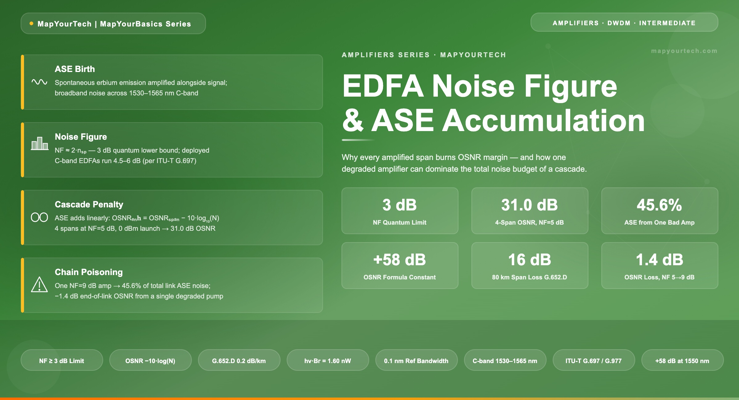
This means a single well-maintained 80 km span at 0 dBm launch power contributes 37 dB of OSNR capacity. Cascading four such spans reduces the end-of-link OSNR to 37 − 10·log10(4) = 37 − 6.02 = 31.0 dB, as derived in Section 6.
For a cascade of N identical spans, ASE powers from all amplifiers add incoherently in the power domain. Total ASE = N × PASE_per_span, which is exactly a factor-of-N increase in noise. Divided into signal power, the OSNR degrades by 10·log10(N) decibels. Double the number of spans, lose 3 dB of OSNR. Quadruple the spans, lose 6 dB.
1 / OSNRtotal (linear) = ∑i=1..N [1 / OSNRspan,i (linear)]
where OSNRspan,i (linear) = 10(OSNRspan,i(dB)/10) for each span i.
This is the exact expression used in planning tools and reproduced in ITU-T G.680 transmission parameter definitions.
The linear summation rule is the mathematical reason a single bad amplifier can dominate the OSNR budget. When ASE powers add as a simple sum, the amplifier with the highest NF — the one with the largest per-span ASE power — contributes proportionally more to the total than its 1/N share. Section 7 quantifies this for a four-span chain with one amplifier at 9 dB NF. For deeper context on how IP-over-DWDM network architectures apply this OSNR budget logic end-to-end across multi-span routes, including the interaction with nonlinear noise contributions, the OSNR cascade approach described here extends to the full GOSNR framework.
6. Four-Span Example: Watching OSNR Degrade
A four-span 320 km link on G.652.D fiber with 80 km spans, 16 dB span loss, and 0 dBm per-channel launch power illustrates the cumulative OSNR penalty in concrete numbers. All four inline EDFAs are set to 16 dB gain. The calculation uses the per-span OSNR formula from Section 5 and the linear summation rule for different NF values.
| Parameter | Value | Notes |
|---|---|---|
| Fiber type | G.652.D (SSMF) | Standard single-mode fiber; ITU-T G.652.D specification |
| Fiber loss coefficient | 0.20 dB/km | Typical deployed loss including splice budget at 1550 nm (specified) |
| Span length | 80 km | Each of 4 spans; total route = 320 km |
| Span loss Lspan | 16 dB | 0.20 dB/km × 80 km (specified) |
| EDFA gain | 16 dB | Set to exactly compensate span loss; AGC mode |
| Per-channel launch power Ps | 0 dBm | Per amplifier output; total WDM power higher depending on channel count |
| Reference bandwidth Bref | 0.1 nm (12.5 GHz) | Standard ITU-T G.697 OSA measurement bandwidth at 1550 nm |
| Optical frequency ν | 193.4 THz | Corresponding to 1550 nm signal wavelength |
The OSNR evolution through the four-span chain, step by step:
| Measurement point | Spans N | OSNR (dB) | 10·log₁₀(N) (dB) | Calculation |
|---|---|---|---|---|
| After EDFA 1 output | 1 | 37.0 | 0.0 | 0 − 5 − 16 + 58 = 37.0 |
| After EDFA 2 output | 2 | 34.0 | 3.0 | 37.0 − 10·log₁₀(2) = 37.0 − 3.01 |
| After EDFA 3 output | 3 | 32.2 | 4.8 | 37.0 − 10·log₁₀(3) = 37.0 − 4.77 |
| After EDFA 4 output (RX) | 4 | 31.0 | 6.0 | 37.0 − 10·log₁₀(4) = 37.0 − 6.02 |
The 31 dB end-of-link OSNR for a well-maintained four-span system sets the baseline. A 400G DP-16QAM coherent channel requires a minimum receiver OSNR of approximately 21–23 dB (vendor-specified per OIF 400ZR IA for 120 km reach; system margin requires 26–28 dB at the line input). The 31 dB baseline leaves approximately 3–4 dB of engineering margin above the 27–28 dB threshold needed for a 400G channel with standard FEC. That margin absorbs connector degradation, splice losses, aging, and — as Section 7 quantifies — any amplifier NF increase.
7. One Noisy Amplifier Poisons the Chain
Replace EDFA 3 in the four-span example with an amplifier whose pump laser has degraded enough to raise the NF from 5 dB to 9 dB — a 4 dB increase reflecting a pump that has lost approximately half its output power over several years of service. The gain is still 16 dB; the span loss compensation is unchanged. Only the ASE injection rate changes.
The per-span OSNR contribution from EDFA 3 drops from 37.0 dB (NF = 5 dB) to 33.0 dB (NF = 9 dB). In linear terms, ASE from EDFA 3 increases from 10−3.70 = 1.995 × 10⁻⁴ to 10−3.30 = 5.012 × 10⁻⁴ relative to the 0 dBm signal — exactly a 10(4/10) = 2.512 factor increase, as the 4 dB NF increase directly predicts.
EDFA 3 (NF = 9 dB): OSNRspan = 33.0 dB → 1/OSNR = 1/1995 = 5.013 × 10⁻⁴
1/OSNRtotal = 3 × 1.995 × 10−4 + 5.013 × 10−4 = 5.985 × 10⁻⁴ + 5.013 × 10−4 = 10.998 × 10⁻⁴
OSNRtotal = 1 / (10.998 × 10⁻⁴) = 909.3 → 10·log₁₀(909.3) = 29.6 dB
End-of-link OSNR drops from 31.0 dB (all-good chain) to 29.6 dB — a 1.4 dB degradation attributable to a single amplifier. The magnitude of this hit depends on how much worse EDFA 3 is relative to the others:
| EDFA 3 NF | EDFA 3 ASE (relative to NF=5 dB) | EDFA 3 share of total ASE | End-of-link OSNR (dB) | OSNR loss vs. all-good (dB) |
|---|---|---|---|---|
| 5 dB (baseline) | 1.00× | 25.0% | 31.0 | 0.0 |
| 7 dB | 1.58× | 35.2% | 30.3 | 0.7 |
| 9 dB | 2.51× | 45.6% | 29.6 | 1.4 |
| 11 dB | 3.98× | 55.7% | 28.8 | 2.2 |
| 13 dB | 6.31× | 67.5% | 27.8 | 3.2 |
The table reveals the non-linear character of single-amplifier degradation. At NF = 11 dB — two degraded pump lasers, not an uncommon failure mode in an aging network — EDFA 3 contributes 55.7% of all link ASE while representing 25% of the amplifier count. At NF = 13 dB, that single amplifier is responsible for two-thirds of total link noise. The other three well-maintained amplifiers are collectively less harmful than the one bad one.
Design risk — correlated margin erosion: A 4 dB NF degradation from pump laser aging (NF 5→9 dB) consumes 1.4 dB of OSNR margin in a four-span link. For a 400G DP-16QAM channel with a 3 dB design margin above the OSNR threshold, this leaves only 1.6 dB remaining. Add fiber aging (0.5 dB over 10 years on typical G.652.D), splice degradation (0.5 dB), and connector contamination (0.5 dB), and the total margin approaches exhaustion before any service-affecting event has occurred. A single 9 dB NF amplifier effectively halves the system's aging headroom.
The physical explanation for this disproportionate impact is direct: ASE powers add linearly, so the amplifier that injects the most ASE dominates the total. In a four-span link with equal span losses and gains, each amplifier's share of total ASE equals its ASE power relative to the sum. A 2.51× increase in one amplifier's ASE shifts the distribution from 25/25/25/25% to 18/18/45.6/18%. The "poison" metaphor in the article's title is accurate: one contaminated amplifier spoils the noise floor that all four amplifiers built together.
Takeaway: ASE from a high-NF amplifier contributes to the end-of-link total in exact proportion to its own ASE spectral density. One amplifier at NF = 9 dB in an otherwise 5 dB chain contributes 45.6% of total link noise and reduces end-of-link OSNR by 1.4 dB. For systems with 3 dB margin, one degraded amplifier erodes nearly half the available headroom — making NF monitoring a first-tier operational priority, not a commissioning-only check.
8. Engineering Implications
8.1 NF Allocation in Link Budget
Link budget analysis for a DWDM route begins with the OSNR target at the receiver and works backward to the maximum tolerable NF per amplifier. For a 320 km four-span system targeting 31 dB end-of-link OSNR, the per-span OSNR budget is 31 + 10·log10(4) = 37.0 dB, requiring NF ≤ 0 − 37.0 + 58 − 16 = 5.0 dB per amplifier at 0 dBm launch power. Relaxing the OSNR target to 30 dB opens the NF budget to 6.0 dB. The relationship is one-to-one: every dB of OSNR target change corresponds to one dB of NF budget change, which is why the line system designer treats NF allocation as a first-order design decision, not a component-level afterthought.
NF allocation also interacts with launch power. A 1 dB increase in per-channel launch power improves OSNR by 1 dB, equivalent to a 1 dB NF improvement — but only up to the point where nonlinear noise (SPM, XPM, FWM) begins to dominate. For an 80 km G.652.D span at 32 Gbaud (100G per channel), this nonlinear threshold sits near −2 to 0 dBm per channel depending on channel count. For a 64 Gbaud (400G) channel, the optimum is typically −1 to +1 dBm. Above those levels, increasing launch power does not improve OSNR — it trades ASE penalty for nonlinear penalty, and the GOSNR (generalised OSNR that accounts for nonlinear interference noise) stays flat or worsens. For analytical tools that model both ASE and nonlinear noise together, the Gaussian Noise model provides the framework for optimising launch power across the full amplifier chain.
8.2 Noise Figure in Pre-Amplifier vs. Inline Configurations
Pre-amplifiers — placed immediately ahead of the receiver terminal or at the input of a reconfigurable add/drop multiplexer (ROADM) — see low input signal power after a long span or passive ROADM loss. At these low input powers, the EDFA operates in its linear (non-saturated) regime, and nsp approaches 1.1–1.2, giving NF near 4–5 dB. The DWDM commissioning process verifies pre-amplifier NF at ≤5 dB as a standard acceptance criterion; inline amplifiers are accepted at NF ≤ 6 dB. Both limits exist because exceeding them at commissioning leaves insufficient margin for the operational life of the system.
Booster amplifiers — placed at the transmitter to raise signal power before fiber entry — add ASE that travels the full link and arrives at the receiver with full accumulation from every subsequent span. A 1 dB NF increase in the booster produces exactly 1 dB of end-of-link OSNR degradation, identical to a 1 dB NF increase in any other amplifier when gain is set to compensate its own loss. The symmetry holds because the formula treats booster ASE the same as ILA ASE: a power that is amplified or attenuated by subsequent elements while the signal power follows the same path.
8.3 Raman Amplification and Effective Noise Figure
Distributed Raman amplification pre-amplifies the signal within the transmission fiber before the lumped EDFA at the end of each span. Because the signal is partially amplified before it reaches its lowest optical power level at mid-span, the EDFA at the span end sees a higher input signal and operates at lower noise contribution. The effective noise figure of the Raman+EDFA combination, expressed as Feff = FEDFA · exp(−αs · L), can fall below 0 dB on the logarithmic scale for sufficient Raman gain — meaning the distributed amplification more than compensates the span loss before the EDFA adds noise. For submarine cable systems and ultra-long terrestrial spans where OSNR budget is tightest, this 3–5 dB effective NF improvement from hybrid Raman+EDFA is often the margin that makes 400G feasible at 120+ km span lengths.
Planning tools for operators managing mixed-vendor, mixed-generation networks must incorporate per-amplifier NF measurements from commissioning records and from periodic OSA sweeps. An EDFA whose NF has drifted 1 dB since commissioning — a realistic trajectory for a pump laser after 5–8 years — contributes 1 dB of unbudgeted OSNR degradation that a static planning model will not detect. For in-house optical link simulation, the article on multivendor planning tools covers how measured NF values are updated in the equipment library to track aging effects in the live network model.
9. Monitoring ASE in Deployed Systems
Optical channel monitors (OCMs) and optical spectrum analysers (OSAs) at amplifier sites measure OSNR in-band or through out-of-band pilots. The in-band measurement — interpolating the noise floor beneath the signal spectrum — requires careful spectral processing because WDM channels are contiguous and the noise floor is obscured by the signal itself. Out-of-band noise monitoring using pilot tones or through periodic OSA sweeps at the line terminals gives a cleaner absolute noise power reading. For DWDM channel monitoring with OCM and OSA, the measurement methodology article details how OSNR measurements in deployed systems account for gain tilt, spectral loading, and filter narrowing effects that can bias in-band OSNR readings.
An OSNR degradation alarm at the receiver terminal does not directly identify which amplifier in the chain is responsible. The standard diagnostic approach traces the OSNR contribution step by step: measure OSNR at each amplifier site's OCM output, apply the per-span formula in reverse to infer each amplifier's NF from its input and output powers, and compare against commissioning baselines. An amplifier whose inferred NF has increased by more than 1.5–2 dB relative to its commissioning value warrants pump laser inspection or replacement.
Scenario: A network monitoring system (NMS) reports end-of-link OSNR of 29.7 dB on a 320 km, four-span route that was commissioned at 31.0 dB. The 1.3 dB degradation exceeds the 1.0 dB alarm threshold. All four spans show unchanged fiber loss on OTDR (no fiber event). Per-channel launch power at 0 dBm is confirmed correct.
Fault isolation: OCM readings at each amplifier site show per-span OSNR contributions of 37.0, 37.0, 33.2, and 37.0 dB for spans 1–4. Span 3 is 3.8 dB below its commissioning value of 37.0 dB, implying NF has risen from ~5.0 dB to ~8.8 dB — consistent with a pump laser that has lost ~3 dB output power from aging. Pump current telemetry at site 3 confirms pump output is 18 mA below specification. Pump laser replacement at site 3 restores OSNR to 30.9 dB (within 0.1 dB of commissioning value, accounting for 0.1 dB of accumulated fiber aging over the service period).
This diagnostic sequence — OCM sweep, per-span NF inference, component-level telemetry confirmation — is the standard resolution path for OSNR degradation events in amplified DWDM networks. The critical enabler is having commissioning baselines for each amplifier's NF, so that a 1 dB drift is detectable against a known reference. Networks without per-amplifier commissioning records must rely on the absolute per-span formula to infer NF from current measurements alone, which introduces uncertainty from span loss changes that may have occurred since installation. Periodic re-measurement of per-span OSNR contributions — ideally during planned maintenance windows every 18–24 months — provides the trending data that predicts pump laser end-of-life before a service-affecting margin event occurs.
For the specific OSNR thresholds that trigger alarms and the NMS configuration that automates these comparisons, the DWDM OSNR monitoring guidelines give alarm threshold values and measurement configuration standards applicable to production networks. The alarm threshold for a single-span OSNR contribution degradation is typically set 2 dB below commissioning value (warning) and 3.5 dB below (critical), leaving response time before the end-of-link OSNR approaches the service threshold for high-order modulation formats.
10. References
- ITU-T G.697 — Optical monitoring for dense wavelength division multiplexing systems. ITU-T Study Group 15.
- ITU-T G.977 — Characteristics of optically amplified submarine cable systems. ITU-T Study Group 15.
- ITU-T G.680 — Physical transfer functions of optical network elements. ITU-T Study Group 15.
- ITU-T G.652 — Characteristics of a single-mode optical fibre and cable. ITU-T Study Group 15.
- OIF-400ZR-01.0 — Implementation Agreement for 400ZR. Optical Internetworking Forum.
- Sanjay Yadav, "Optical Network Communications: An Engineer's Perspective" — Bridge the Gap Between Theory and Practice in Optical Networking.

Optical Communications & Network Automation Expert | Author of 3 Books for Optical Engineers | Founder, MapYourTech
Optical networking engineer with nearly two decades of experience across DWDM, OTN, coherent optics, submarine systems, and cloud infrastructure. Founder of MapYourTech. Read full bio →
Follow on LinkedIn