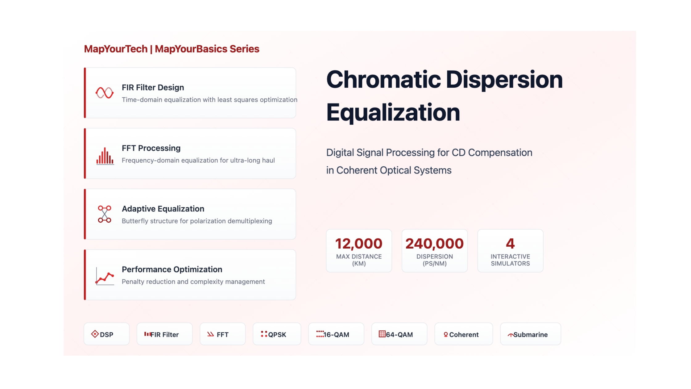

Chromatic Dispersion Equalization
Fundamentals & Core Concepts
What is Chromatic Dispersion Equalization?
Chromatic Dispersion (CD) Equalization is a digital signal processing technique used in coherent optical communication systems to compensate for the frequency-dependent group delay that occurs when optical signals propagate through fiber. As different wavelength components of an optical signal travel at different speeds through the fiber, the signal becomes temporally dispersed, causing inter-symbol interference (ISI) and degrading system performance.
Why Does Chromatic Dispersion Occur?
Chromatic dispersion arises from the frequency-dependent refractive index of optical fiber. This phenomenon causes different spectral components of a signal to experience different propagation delays. The effect can be modeled by the following differential equation:
Where:
• E: Electric field envelope
• z: Propagation distance (km)
• β₂: Group velocity dispersion parameter (ps²/km)
• t: Time in moving frame (ps)
When Does CD Equalization Matter?
- Long-haul transmission: Distances exceeding 80 km require CD compensation
- High baud rate systems: 35 Gbaud and higher signals are more sensitive to dispersion
- Green field deployments: Digital CD compensation eliminates the need for optical dispersion compensating fiber (DCF)
- Ultra-long submarine systems: Transmission lengths up to 12,000 km with accumulated dispersion exceeding 240,000 ps/nm
Why is CD Equalization Important?
CD equalization is one of the most important enabling technologies for modern high-capacity optical networks:
- Cost Reduction: Eliminates expensive optical dispersion compensation modules
- Flexibility: Enables dynamic adaptation to varying fiber types and distances
- System Performance: Enables higher-order modulation formats (16-QAM, 64-QAM) over long distances
- Nonlinearity Mitigation: Large dispersion during propagation reduces self-phase modulation and cross-phase modulation effects
- Network Simplification: Removes the need for precise dispersion management in the optical layer
Mathematical Framework
Frequency Domain Transfer Function
The most computationally efficient approach to CD compensation is solving the dispersion equation in the frequency domain. Taking the Fourier transform of the propagation equation yields:
For compensation, the equalizer applies the inverse:
H_CD(z, ω) = exp[-(j/2) × β₂ × ω² × z] = F_CD(-z, ω)
Where:
• ω: Angular frequency (rad/s)
• z: Link length (km)
• β₂: GVD parameter (ps²/km)
Time Domain Impulse Response
The impulse response can be obtained via inverse Fourier transform:
Where: φ(t) = t²/(2β₂z)
This represents a chirped impulse with quadratic phase variation.
Relationship Between Dispersion Parameters
The dispersion coefficient D and group velocity dispersion β₂ are related:
Temporal spread calculation:
Δt = D × z × Δλ
Where:
• D: Dispersion coefficient (ps/nm/km)
• c: Speed of light (3×10⁸ m/s)
• λ: Wavelength (nm)
• Δλ: Spectral width (nm)
• Δt: Temporal spread (ps)
Standard SMF-28: D ≈ 17 ps/nm/km at 1550 nm
FIR Filter Tap Calculation
For digital implementation using Finite Impulse Response (FIR) filters, the minimum number of taps required depends on the accumulated dispersion:
Or equivalently:
N_taps ≈ 0.27 × B_s² × D × L / 1000
Where:
• T_s: Sampling period (s)
• B_s: Symbol rate (Gbaud)
• D: Dispersion coefficient (ps/nm/km)
• L: Link length (km)
Practical Calculation Example
Given:
• Symbol rate: 35 Gbaud
• Link length: 1000 km
• Dispersion: D = 17 ps/nm/km
• Sampling: 2 samples per symbol
Step 1: Calculate spectral width
Δλ = (35 GHz) × (8 pm/GHz) = 0.28 nm
Step 2: Calculate temporal spread
Δt = 17 × 1000 × 0.28 = 4,760 ps
Step 3: Calculate symbol periods spread
Symbol period = 1/35 Gbaud = 28.6 ps
Spread = 4,760 / 28.6 ≈ 166 symbols
Step 4: Required taps (T/2 spaced)
N_taps ≈ 2 × 166 ≈ 332 taps
Manageable complexity for modern DSP
Types & Components
Classification of CD Equalization Approaches
| Type | Domain | Best Use Case | Complexity |
|---|---|---|---|
| Time-Domain FIR | Time | Short to moderate dispersion (<50,000 ps/nm) | O(N) per sample |
| Frequency-Domain FFT | Frequency | Large dispersion (>50,000 ps/nm) | O(N log N) per block |
| Overlap-and-Save | Frequency | Ultra-long haul (submarine systems) | Most efficient for large N |
| Overlap-and-Add | Frequency | Block processing applications | Similar to overlap-and-save |
Time-Domain FIR Filter Equalization
Truncated Impulse Response Design
The simplest approach truncates the infinite impulse response to a finite window:
- Tap weights: h_TI[n] = (1/√ρ) × exp(-jπ/ρ × (n - (N-1)/2)²)
- Parameter: ρ = 2πβ₂z/T_s²
- Advantages: Simple closed-form solution, intuitive design
- Limitations: Aliasing effects, performance degrades with high-order modulation
Least Squares FIR Design
Optimizes tap weights to minimize mean square error:
- Method: Band-limits signal to Nyquist frequency before truncation
- Window function: Uses error function (erfi) for optimal shaping
- Advantages: Significantly reduced penalty, better for higher-order modulation
- Flexibility: Can increase taps beyond minimum to further reduce penalty
Frequency-Domain FFT-Based Equalization
Implementation Steps
- FFT: Convert time-domain signal to frequency domain
- Multiply: Apply H_CD(β₂, ω, L) = exp(-jβ₂ω²L/2)
- IFFT: Convert back to time domain
Block Processing: Uses overlap-and-save or overlap-and-add algorithms to handle continuous data streams efficiently.
Most efficient for submarine systemsComponent Breakdown
| Component | Function | Characteristics |
|---|---|---|
| Static CD Equalizer | Compensates bulk chromatic dispersion | Large filter size, virtually static, implemented in frequency domain |
| Adaptive Butterfly Equalizer | Polarization demux, PMD compensation, residual CD | Shorter filters, time-varying, uses CMA or LMS algorithms |
| Clock Recovery | Symbol timing synchronization | Operates after CD compensation |
| Carrier Recovery | Frequency offset and phase estimation | Final stage before symbol decision |
Comparison: Time vs. Frequency Domain
- Lower latency for short dispersion
- Simpler implementation
- Direct tap coefficient calculation
- Dramatically lower complexity for large dispersion (40% of DSP power in submarine systems)
- Handles ultra-long haul (up to 12,000 km)
- More efficient for accumulated dispersion > 100,000 ps/nm
Effects & Impacts
System-Level Effects of Uncompensated CD
Inter-Symbol Interference (ISI)
Primary degradation mechanism where temporal spreading causes adjacent symbols to overlap:
- Pulse broadening: Signal energy spreads beyond symbol period
- Eye diagram closure: Reduced eye opening degrades BER performance
- Sensitivity penalty: Requires higher OSNR to achieve target BER
Modulation Format Sensitivity
Higher-order modulation formats are more susceptible to residual dispersion:
- QPSK: Relatively robust, tolerates imperfect compensation
- 16-QAM: Moderate sensitivity, requires good equalization
- 64-QAM: Highly sensitive, demands excellent equalization (penalty > 2.5 dB without proper filter design)
Performance Implications
| Distance | Accumulated Dispersion | QPSK Penalty | 64-QAM Penalty |
|---|---|---|---|
| 20 km | 340 ps/nm | < 0.1 dB | ~0.5 dB |
| 200 km | 3,400 ps/nm | < 0.5 dB | ~1.5 dB |
| 2000 km | 34,000 ps/nm | < 1.0 dB | ~2.5 dB |
| 12,000 km | 240,000 ps/nm | ~1.5 dB | > 3.0 dB |
Penalties shown for truncated impulse response design at BER = 2×10⁻²
Equalization-Enhanced Phase Noise (EEPN)
EEPN Mechanism
When compensating large amounts of dispersion, the phase noise of the local oscillator is amplified by the all-pass CD transfer function:
- Impact: Additional OSNR penalty beyond simple CD compensation
- Mitigation: Use lasers with narrow linewidth (< 100 kHz)
- Submarine systems: With linewidth < 100 kHz, EEPN remains acceptable even after 10,000 km
Tolerance Levels and Thresholds
| System Type | Max CD Tolerance | Typical Operating Range |
|---|---|---|
| Metro (10G) | ~1,000 ps/nm | 0-800 ps/nm |
| Regional (100G) | ~50,000 ps/nm | 0-35,000 ps/nm |
| Long-haul (100G+) | ~100,000 ps/nm | 20,000-80,000 ps/nm |
| Submarine (100G+) | ~300,000 ps/nm | 100,000-250,000 ps/nm |
Mitigation Strategies Overview
- Frequency-domain FFT-based equalization for large dispersion
- Least squares FIR design for improved performance with high-order modulation
- Increasing tap count beyond minimum to reduce penalty
- Split compensation between transmitter and receiver DSP
- Dispersion Compensating Fiber (DCF) modules
- Fiber Bragg Grating (FBG) compensators
- Dispersion management in WDM systems
- Allow large in-line dispersion to mitigate fiber nonlinearities
- Use narrow linewidth lasers to minimize EEPN
- Select appropriate modulation format for link distance
Interactive Simulators
Practical Applications & Case Studies
Real-World Deployment Scenarios
Case Study 1: Trans-Atlantic Submarine System
Challenge:Deploy 100G PDM-QPSK over 6,000 km with accumulated dispersion of 126,000 ps/nm without optical dispersion compensation.
Solution Approach:
- Frequency-domain FFT-based CD equalization using overlap-and-save algorithm
- FFT block size: 2048 samples to handle large dispersion
- Narrow linewidth lasers (< 100 kHz) to minimize EEPN
- Adaptive butterfly equalizer with 17 taps for PMD compensation
- CD compensation consumed ~38% of total DSP power
- Processing latency: ~15 microseconds
- Achieved OSNR penalty < 1.2 dB for CD+EEPN combined
Successfully deployed system with BER < 2×10⁻² before FEC, providing error-free transmission after FEC. Eliminated need for 30+ in-line DCF modules, saving significant cost and reducing system complexity.
Highly Successful
Case Study 2: Metro Network Upgrade to 400G
Challenge:Upgrade existing metro network from 100G to 400G (35 Gbaud PDM-16QAM) over mixed fiber types with varying dispersion (8-21 ps/nm/km) and distances up to 120 km.
Solution Approach:
- Implemented least squares FIR design with 66% tap overhead
- Dynamic dispersion estimation during startup using blind search
- Matched filter design integrated into CD equalizer
- Reduced adaptive equalizer complexity from 25 to 13 taps
- Maximum accumulated dispersion: 2,520 ps/nm (120 km × 21 ps/nm/km)
- Required FIR taps: minimum 53, actual 88 (with overhead)
- CD equalization penalty: < 0.5 dB across all fiber types
Achieved seamless upgrade without fiber replacement. Total system penalty including CD equalization, adaptive filtering, and carrier recovery remained under 2.5 dB. Network capacity increased 4× while maintaining same reach.
Cost-Effective Solution
Case Study 3: High-Capacity Data Center Interconnect
Challenge:Deploy 800G (64 Gbaud PDM-64QAM) over 80 km of ultra-low-loss fiber (ULLF) for data center interconnection requiring minimal latency.
Solution Approach:
- Optimized least squares FIR with extended tap count (120% of minimum)
- Parallel FIR implementation with 256-way parallelism
- Low-latency design: time-domain equalization to minimize processing delay
- Integrated matched filtering in CD equalizer to simplify adaptive stage
- Accumulated dispersion: 1,360 ps/nm (80 km × 17 ps/nm/km)
- Required taps: minimum 279, implemented 335
- Total DSP latency: < 5 microseconds
- Achieved penalty < 0.3 dB for 64-QAM constellation
Successfully deployed ultra-high-capacity links with 800 Gb/s per wavelength. The optimized CD equalization enabled reliable 64-QAM transmission while maintaining low latency requirements. System operates with 2 dB margin to FEC threshold.
High Performance
Troubleshooting Guide
| Problem | Possible Cause | Solution |
|---|---|---|
| High BER after equalization | Incorrect dispersion estimation | Re-run blind dispersion search algorithm; verify fiber type and length |
| Constellation distortion | Insufficient FIR taps | Increase tap count by 50-100%; switch to frequency-domain for large dispersion |
| Phase noise degradation | EEPN from wide linewidth LO | Use narrow linewidth laser (<100 kHz); consider split compensation |
| Slow convergence | Adaptive equalizer starting point | Initialize butterfly equalizer with identity matrix; adjust CMA step size |
| Performance varies with modulation | Truncated IR filter design | Switch to least squares design; increase overhead taps for higher-order QAM |
| High DSP power consumption | Oversized time-domain filter | Implement FFT-based frequency domain equalization for dispersion >50,000 ps/nm |
Quick Reference Tables
Recommended Filter Design by Application
| Application | Distance | Modulation | Recommended Approach |
|---|---|---|---|
| Metro/Regional | < 200 km | QPSK/16-QAM | Time-domain FIR, truncated IR acceptable |
| Long-haul | 200-2000 km | 16-QAM/64-QAM | Time-domain FIR, least squares design |
| Ultra-long haul | 2000-6000 km | QPSK/16-QAM | Frequency-domain FFT, overlap-and-save |
| Submarine | > 6000 km | QPSK | Frequency-domain FFT, large block size |
Professional Recommendations
- Always use least squares design for 16-QAM and above - The penalty reduction justifies the marginally increased complexity
- Budget 50-100% tap overhead for high-order modulation - Extra taps dramatically reduce penalty for 64-QAM
- Switch to frequency domain above 50,000 ps/nm - Computational efficiency gain becomes significant
- Use narrow linewidth lasers (<100 kHz) - Essential for submarine and ultra-long haul to control EEPN
- Implement blind dispersion estimation - Allows flexible deployment across varying fiber plants
- Partition equalization between CD and adaptive stages - Optimize each for its specific task (static vs dynamic)
- Consider split compensation for ultra-long haul - Distribute CD compensation between Tx and Rx to manage DSP complexity
- Integrate matched filtering with CD equalization - Reduces complexity of subsequent adaptive equalizer
- Allow large in-line dispersion - Counterintuitively reduces fiber nonlinear impairments
- Test across full operating range - Validate performance at extremes of temperature, OSNR, and dispersion
- ASIC Design: Parallel FIR implementation essential for high-speed operation (e.g., 256-way parallelism for 35 Gbaud)
- Memory Requirements: FFT-based approaches require substantial buffer memory for block processing
- Latency vs Complexity: Time-domain offers lower latency but higher complexity for large dispersion
- Power Budget: CD compensation can consume 30-40% of total receiver DSP power in submarine systems
- Acquisition Time: Blind dispersion search typically completes in 100-500 microseconds

Optical Communications & Network Automation Expert | Author of 3 Books for Optical Engineers | Founder, MapYourTech
Optical networking engineer with nearly two decades of experience across DWDM, OTN, coherent optics, submarine systems, and cloud infrastructure. Founder of MapYourTech. Read full bio →
Follow on LinkedIn