
MapYourTech | InDepth Series
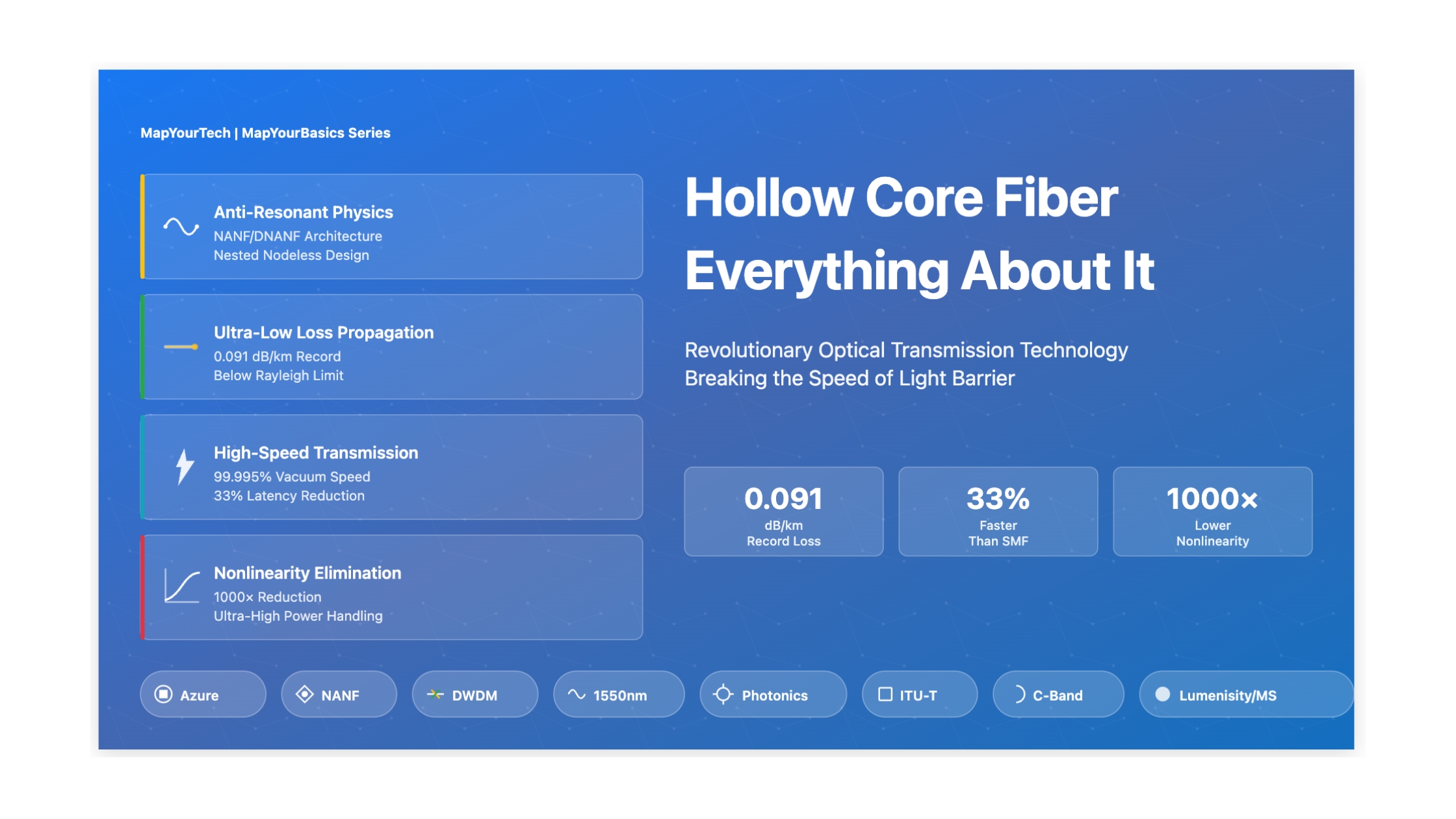
Hollow Core Fiber: Everything About It
An engineering analysis of how air-guided light breaks the silica Rayleigh limit, the loss and dispersion numbers behind it, and where the cost premium is worth paying.
1. Executive Summary
1.1 Key Findings
Attenuation below the silica scattering floor
Hollow Core Fiber (HCF) has measured an attenuation of 0.091 dB/km at 1,550 nm, published in Nature Photonics, taking it below the 0.142 dB/km Rayleigh scattering floor that bounds solid silica. This is the first time an optical fiber has carried a signal with lower loss than the best possible solid glass over the telecom band. It guides the signal through air rather than glass, so the loss mechanism that limits conventional fiber no longer applies. The work that produced it grew out of the physics of guiding light in air rather than any improvement in glass purity.
Light travels through HCF at about 99.995% of vacuum speed (effective index near 1.0003) against roughly 66% in solid glass. That single property produces the measurable advantages engineers care about:
- Unamplified reach: spans extend roughly 1.5× without amplification (about 33 km versus 15–20 km on SMF) because the per-km loss is lower.
- Chromatic dispersion: below 3 ps/(nm·km), about 7× lower than SMF, which lightens the DSP equalizer load.
- Polarization mode dispersion: 0.004–0.016 ps/√km in NANF designs against ≤0.20 ps/√km for SMF.
- Power handling: 1.2 Tbit/s carried at 3 W launch power with no measurable nonlinear penalty — a China Telecom demonstration.
1.2 Approach
This analysis draws together laboratory results, field-deployment reports, and manufacturing data, then verifies every quantitative claim against published sources. Four dimensions structure the work:
| Analysis dimension | Source type | Key metrics |
|---|---|---|
| Laboratory performance | Peer-reviewed journals, conference digests | Attenuation, dispersion, PMD, spectral response |
| Field deployments | Hyperscaler and carrier deployment reports | Splice loss, BER, reliability, uptime |
| Manufacturing capability | Producer and partnership announcements | Continuous length, yield, production volume |
| Economics | Market studies, deployment cost reporting | Cost per meter, total cost of ownership, return on investment |
1.3 Conclusions
Strategic market position
HCF has moved from laboratory demonstration to deployed infrastructure, reaching Technical Readiness Level 9 for specialized routes. Adoption stays inside niche markets where the performance advantage pays for the 50–100× cost premium over conventional fiber ($5–10/meter against roughly $0.10/meter for high-volume SMF).
Commercial viability separates sharply by application:
| Application | Deployment status | Value proposition | Market penetration |
|---|---|---|---|
| High-frequency trading | Production (3+ years) | Microsecond head-starts convert into trading profit | Established |
| AI data center interconnect | Active deployment | 2.25× larger area for facility siting at fixed latency | Growing |
| Hyperscale cloud | Microsoft: 15,000 km planned | Differentiated ultra-low-latency services | Early adoption |
| Telecommunications | Trial phase | 5G/6G fronthaul latency budget, lower power | Pilot projects |
| FTTH / consumer | Not viable | Cost prohibitive; installed-base inertia | None |
Four conditions gate mainstream adoption: an order-of-magnitude manufacturing cost reduction; ITU-T recommendations equivalent to the G.652/G.654/G.655 series; a multi-vendor support base with standardized test equipment and trained field technicians; and HCF-SMF splice loss cut from today's 0.3–0.6 dB toward below 0.15 dB. Market projections put growth from $10–20 million in 2024 to between $916 million and $3.17 billion by 2032–2033, a compound annual growth rate of 24–27.4%.
Takeaway: HCF is proven and deployed, but only where a microsecond or a megawatt of siting flexibility is worth a 50–100× cost premium. The physics advantage is settled; the economics are the gate.
2. Introduction and Background
2.1 The Physical Limits of Silica Fiber
Single-mode fiber confines light in a solid glass core by total internal reflection, and that one principle carried global telecommunications for over fifty years. By 2020 the technology sat against limits set by the silica glass itself, not by manufacturing skill.
2.1.1 The Rayleigh Scattering Floor
Rayleigh scattering sets the minimum attenuation of silica at 1,550 nm to 0.142 dB/km — a consequence of microscopic density fluctuations frozen into the glass during the draw. No purification removes them; they are part of how amorphous glass forms. Production SMF-28 reaches 0.14–0.20 dB/km, approaching this floor but never crossing it.
2.1.2 Latency in Glass
Light moves through silica at roughly 66% of vacuum speed (effective index ~1.467), which adds about 4.9 µs/km of propagation delay. For high-frequency trading, distributed AI training, and tactile-internet workloads that budget in microseconds, that delay is a hard ceiling. It also caps how far apart synchronized data centers can sit — about 60 km for millisecond-level coordination on SMF.
2.1.3 Nonlinear Effects and Power Scaling
The Kerr nonlinearity of silica (n₂ ≈ 2.6 × 10⁻²⁰ m²/W) shows up as a family of power-dependent impairments in fiber:
- Self-phase modulation (SPM): intensity-dependent phase distortion on the channel itself.
- Cross-phase modulation (XPM): one channel's power shifts the phase of its neighbors.
- Four-wave mixing (FWM): mixing products land on other channels as interference.
- Stimulated Brillouin scattering (SBS): backscatter that caps launch power near 10–13 dBm.
- Stimulated Raman scattering (SRS): power transfer from short to long wavelengths across the band.
Together these set strict per-channel power limits that bound capacity and reach. Across a wide S+C+L window of more than 15 THz, SRS tilts the spectrum hard — L-band channels gain several dB while S-band channels deplete — so a flat GSNR is impossible without active compensation. The same effect drives the design rules behind C+L band DWDM systems.
2.2 Problem Statement: Demand Outruns the Material
The AI-driven infrastructure constraint
Training large models networks thousands of GPUs into clusters where communication latency directly bounds compute efficiency. On conventional fiber a synchronized training cluster keeps facilities within about 60 km to hold millisecond-level coordination. That forces operators to pack compute into power-constrained urban sites, and the resulting power ceiling bounds how far a single training run can scale.
The performance targets that SMF cannot meet are specific:
| Application domain | Latency requirement | Bandwidth requirement | SMF limitation |
|---|---|---|---|
| High-frequency trading | <1 µs/km round-trip | 10–100 Gbps | Cannot reach sub-microsecond per km |
| Distributed AI training | <100 µs cluster-wide | 100+ Tbps aggregate | Geographic limit caps power access |
| 5G/6G fronthaul | <100 µs | 25–100 Gbps per radio unit | Fiber consumes the latency budget |
| Quantum communications | Not latency-bound | Photon-level | Polarization drift, high loss |
2.3 Objectives: Performance Through Architecture
HCF answers these limits by changing the guidance mechanism rather than the glass. It confines the signal in an air core using a microstructured cladding that forms a photonic bandgap or anti-resonant reflection, putting over 99% of the optical power in air. Four targets follow directly:
Each target opens network designs that silica physics had closed. The move from demonstration to deployed infrastructure marks the decisive point in this technology's history.
Takeaway: SMF hit three walls at once — the Rayleigh loss floor, the 66%-of-c latency penalty, and the Kerr nonlinearity power ceiling. HCF removes all three by putting the light in air instead of glass.
3. Technical Analysis
3.1 Light Guidance Mechanisms
HCF abandons total internal reflection, the rule behind conventional fiber. It confines light in an air core (n ≈ 1.0) using a microstructured cladding that forms either a photonic bandgap or anti-resonant reflection, so more than 99% of the optical power propagates through air. That single structural change drives every performance number in this article.
3.1.1 Photonic Bandgap Fiber (PBGF)
The first HCF generation used the photonic bandgap effect, drawn from photonic-crystal theory. A periodic cladding microstructure — usually a triangular lattice of air holes in silica — forms a two-dimensional photonic crystal with spectral regions where propagation inside the cladding is forbidden.
PBGF structure
- Periodic honeycomb lattice of air holes
- 7-cell or 19-cell hollow core defect
- Strict periodicity requirement
- Silica struts between air holes
Operating principle
- Bandgap in the cladding traps light in the core
- Light inside the gap cannot escape
- Strong confinement within the operating band
- Sensitive to structural imperfection
Early PBGF designs reached 1.2–1.7 dB/km in the C-band, proving HCF viable. Their limits were the bandgap width (about 100–200 nm of usable spectrum), surface modes at the core-cladding interface that ate into that bandwidth, and a fabrication tolerance so tight that hole-size and position errors degraded performance over kilometer lengths.
3.1.2 Anti-Resonant Fiber (ARF)
The anti-resonant reflection principle
ARF confines light by thin-film interference instead of periodic structures. Thin glass membranes around the core act as Fabry-Pérot resonators set transverse to the fiber axis. Light at wavelengths that resonate with the wall couples into the cladding and leaks; light at anti-resonant wavelengths reflects strongly and stays in the air core.
Anti-resonance holds when the optical thickness of the glass wall sits away from integer multiples of a half-wavelength. The confinement loss scales as:
Two design rules fall out of that scaling: a larger core diameter cuts confinement loss with the cube of D, and tuned wall thickness opens broad anti-resonant bands.
3.1.3 Nested Anti-Resonant Nodeless Fiber (NANF) — Leading Architecture
The NANF design, developed at the University of Southampton, is the current best-performing HCF. It carries two structural ideas:
Nodeless geometry: in earlier ARF designs the capillaries touched, and those contact points (nodes) acted as resonant leakage paths that punched narrow loss peaks into the transmission window. Separating the capillaries completely yields a smooth, wide, low-loss spectrum across octave bandwidths.
Nesting: placing smaller secondary capillaries inside the primary tubes adds anti-resonant reflecting surfaces without adding structural complexity, cutting confinement loss by an order of magnitude against simple ARF.
NANF performance evolution
Early HCF prototypes lost 5 dB/m — only 30% of the light survived a single meter. NANF improved that by a factor of 10,000×, reaching 5 dB over 10 km. That is a reduction from 5,000 dB/km to 0.5 dB/km, and then to the current 0.091 dB/km record.
3.1.4 Double-Nested NANF and Advanced Geometries
Double-Nested Anti-Resonant Nodeless Fiber (DNANF) adds a third nesting level — smaller tubes inside the secondary capillaries. This geometry produced a 0.174 dB/km result, directly comparable to SMF-28, and underpins the proprietary designs behind current commercial deployments. Three refinements push it further:
- Fourfold truncated DNANF: truncated outer tubes suppress higher-order modes (HOMER >1000 dB/km) while holding fundamental-mode loss below 0.2 dB/km.
- Negative-curvature design: core-facing surfaces bow outward, pushing the optical field off the glass and cutting surface scattering to under 15% of total attenuation.
- Multi-size anti-resonant elements: varied tube diameters tune bend performance to 0.18 dB/m at a 0.75 cm radius.
3.2 System Architecture
3.2.1 From Preform to Deployed Fiber
HCF is made by stack-and-draw, not the modified chemical vapor deposition used for conventional fiber. The process trades the smooth chemistry of MCVD for hand assembly of micron-precise glass tubes:
| Stage | Process | Critical parameters | Challenge |
|---|---|---|---|
| Capillary fabrication | Glass tubes drawn to exact dimensions | Wall 200–600 nm, diameter ±0.5 µm | Micron precision over meter lengths |
| Preform assembly | Manual stacking in precise geometry | Rotational alignment 0.1°, sub-micron gaps | Labor-intensive, contamination-sensitive |
| Consolidation | Heat-fuse the outer jacket without collapsing structure | Temperature-gradient and pressure control | Keeping the microstructure intact |
| Fiber draw | Continuous pull through a furnace | Draw 5–20 m/min, tension and diameter control | Yield <70% vs. >95% for SMF |
| Coating & cabling | Polymer coat, hermetic seal, cable assembly | Helium leak rate <10-12 atm·cc/s | Blocking moisture and contamination |
Current production capability spans several producers: continuous lengths above 15 km holding specification end-to-end at the UK draw facility; a 21.7 km continuous supporting-tube HCF at 0.05 dB/km; a Corning manufacturing partnership applying North Carolina precision-fiber capacity; and a European glass producer adapting telecom-scale capacity for HCF.
3.2.2 Loss Mechanisms and Mitigation
Total loss splits into mechanisms that each need a specific design answer. In a typical NANF, confinement dominates while surface scattering and material absorption follow:
| Mechanism | Physical origin | Typical share | Mitigation |
|---|---|---|---|
| Confinement loss | Mode-field overlap with the cladding | 60–80% | Nesting, larger cores, tuned wall thickness |
| Surface scattering | Roughness at glass-air interfaces (1–5 nm RMS) | 15–30% | Negative curvature, surface treatment, less glass overlap |
| Material absorption | Silica intrinsic absorption, impurities | 5–10% | High-purity silica, minimal glass interaction |
| Bend loss | Mode deformation raises cladding coupling | Deployment-dependent | Multi-size anti-resonant elements, controlled radii |
| Water vapor | Absorption at 1364 nm | 0 to severe | Hermetic seal, nitrogen/argon purge at 100 kPa |
Water vapor: the dominant operational risk
Water vapor is the most severe field risk. Concentrations of 18–22 g/m³ raise attenuation at 1364 nm across about 90 nm of bandwidth at ≥0.2 dB/km. One photonic bandgap fiber lost 10 dB after 10 months at 40% relative humidity and 22°C. NANF designs with 250:1 lower glass overlap resist it better, but hermetic sealing with inert-gas purge stays mandatory — and holding that seal during outdoor splicing is what tests an installation crew.
3.3 Performance Metrics
3.3.1 Attenuation: Below the Rayleigh Floor
Crossing the silica Rayleigh floor is the headline result. The measured numbers, by source class:
HCF also reaches across spectral windows silica cannot serve well:
- Telecom (1530–1625 nm): competitive with SMF in C/L, so DWDM equipment works.
- Visible (660 nm): 2.85 dB/km — 71% below the silica Rayleigh value — opening quantum links.
- Wide window: a 66 THz low-loss band from 700 nm past 2,400 nm against silica's narrow telecom sweet spot.
- Multi-octave: one design covers O-band through L-band without wavelength-specific tuning.
3.3.2 Latency and Propagation Speed
HCF carries the signal at 99.995% of vacuum speed (neff ≈ 1.0003) against 66% in solid glass (neff ≈ 1.467):
| Scenario | Distance | SMF round-trip | HCF round-trip | Advantage |
|---|---|---|---|---|
| Trading exchange link | 10 km | 98 µs | 66.8 µs | 31.2 µs |
| Data center interconnect | 90 km | 882 µs | 601.2 µs | 280.8 µs |
| Metro network | 40 km | 392 µs | 267.2 µs | 124.8 µs |
| 5G fronthaul | 15 km | 147 µs | 100.2 µs | 46.8 µs |
3.3.3 Chromatic Dispersion and PMD
HCF carries far less dispersion than conventional fiber, which lightens the receiver DSP load. The comparison is direct:
Conventional SMF
- Chromatic dispersion: ~17 ps/(nm·km) at 1550 nm
- PMD: ≤0.20 ps/√km typical
- Needs heavy DSP equalization
- Constrains modulation order and reach
Hollow Core Fiber
- Chromatic dispersion: <3 ps/(nm·km) — 7× lower
- PMD: 0.004–0.016 ps/√km in NANF
- Lighter DSP, lower power
- Higher-order modulation with less penalty
The low PMD comes from 8-tube geometries with 90° rotational symmetry, where only 0.001–0.03% of the light touches glass. PMD removal is one of HCF's clearest wins in coherent systems — it eliminates a statistical impairment that conventional links must track continuously, the same way dispersion slope across a wide DWDM band shapes design margins.
3.3.4 Nonlinearity
1000× lower nonlinearity
The HCF nonlinear coefficient γ ≈ 0.001 W-1km-1 is about three orders of magnitude below SMF (γ ≈ 1.3 W-1km-1). With nonlinearity off the table, the system limit moves to amplifier noise and terminal electronics — a different design regime entirely.
The field demonstrations bear this out:
- High power: 1.2 Tbit/s single-wavelength at 3 W (34.8 dBm) with no nonlinear penalty — a China Telecom result.
- Extended reach: 301.7 km unrepeated, letting a network skip one amplifier site in every two or three.
- WDM density: over 100 Tbps aggregate on one fiber with no four-wave mixing or cross-phase modulation.
- Coherent: 64-QAM and probabilistic constellation shaping run without nonlinear distortion.
Removing SBS and FWM lifts the power-scaling ceiling that bounds conventional fiber, which matters most in wideband multiband transmission.
Takeaway: NANF and its double-nested variants win because they attack confinement loss, the dominant mechanism. Larger air cores, nodeless geometry, and nested reflecting walls together carry the loss below silica's floor while cutting dispersion, PMD, and nonlinearity at the same time.
4. Implementation Details
4.1 Design Considerations
A working HCF deployment needs system-level planning across infrastructure fit, field procedure, and performance margin. The framework below comes from production deployments.
4.1.1 Network Architecture Planning
| Design element | Requirement | Consideration | Practice |
|---|---|---|---|
| Route planning | Minimize bends, plan splice points | Bend radius >30 cm preferred; access every 200–400 m | Reuse existing conduit; plan underground joints |
| Hybrid architecture | HCF-SMF interface points | Each interface adds 0.3–0.6 dB | Minimize transitions; use mode-field adapters and GRIN bridges |
| Amplifier spacing | Extended reach | 1.5× longer spans (33 km vs. 20 km) | Drop amplifier sites where the power budget allows |
| DWDM integration | Standard equipment fit | Lower dispersion lightens DSP; low nonlinearity allows higher power | Use the wide spectral window; tune per-channel launch power |
| Monitoring | HCF-specific OTDR | 40 dB lower backscatter than SMF | Deploy HCF OTDR; set a baseline; monitor continuously |
Amplifier spacing follows from the loss budget; the same OSNR accounting across an amplified cascaded span applies, except the lower HCF loss per km buys longer reach between sites.
4.1.2 Splice Engineering
Splice loss management
Splice loss is the dominant deployment challenge. HCF-HCF joints reach 0.05–0.16 dB, but HCF-SMF interfaces cost 0.3–0.6 dB each. One hyperscaler field deployment held a mean splice loss of 0.16 dB with individual splices as low as 0.04 dB using purpose-built equipment and procedure. The interoperability between standard SMF and HCF at these joints is where most of the budget is spent.
| Splice type | Technology | Typical loss | Back-reflection | Application |
|---|---|---|---|---|
| HCF-HCF fusion | Ring-of-fire fusion splicer | 0.05–0.16 dB | Moderate | Production deployment |
| HCF-SMF with GRIN | Graded-index multimode bridge | 0.3–0.6 dB per joint | Low with AR coating | Mode-field matching |
| Angle-cleaved | 4.5–8° cleave with offset | 0.6–1.2 dB | <-64 dB | Coherent, low-reflection links |
| Reverse-taper SMF | Thermally expanded SMF core | 0.44 dB per interface | Variable | Lab / prototype |
| Connectorized patch | LC/FC/SC adapters | <0.3 dB | Manageable | Inside plant, patch panels |
4.2 Best Practices
4.2.1 Installation
Hyperscaler deployment experience set field methods now used as benchmarks:
- Blown-fiber install: high-pressure air into pre-installed conduit, holding the hermetic seal throughout.
- Cable handling: hybrid cables (32 HCF + 48 SMF strands) need controlled bend radius and protected routing.
- Joint enclosures: custom underground chambers house fusion splices with environmental protection and access.
- Hermetic sealing: nitrogen/argon purge at 100 kPa overpressure; leak rate <10⁻¹² atm·cc/s.
- Test protocol: HCF-specific OTDR characterization, splice-loss verification, 24+ days of operational monitoring, continuous BER tracking. The same approach applies to an OTDR deep dive for hollow core fiber, where the 40 dB lower backscatter changes how traces read.
4.2.2 Performance Validation
4.3 Common Pitfalls and Mitigation
| Pitfall | Consequence | Mitigation | Prevention |
|---|---|---|---|
| Water vapor ingress | 10 dB+ spike at 1364 nm | Hermetic re-seal, nitrogen purge | Strict sealing, continuous monitoring |
| Excess splice loss | Link budget exhausted, reach lost | Re-splice with tuned parameters | Technician training, alignment checks |
| Bend-induced loss | Attenuation rise >1 dB | Route correction, protective enclosure | Route planning, bend-radius enforcement |
| Higher-order-mode excitation | Modal noise, signal degradation | Launch conditioning, mode filtering | Precise coupling, quality connectors |
| Contamination | Scattering loss, performance drift | Clean-room re-termination | Sealed end caps, clean handling |
Takeaway: The fiber works; the joints and the seal decide whether a deployment succeeds. Budget the HCF-SMF interface loss explicitly, invest in fusion equipment and technician training, and treat hermeticity as a continuous monitoring task, not a one-time install step.
5. Case Studies and Applications
5.1 Industry Examples
Case Study 1: Hyperscale Cloud Infrastructure
Background: After acquiring a hollow-core fiber innovator, a major hyperscaler began the largest HCF deployment to date, targeting global cloud infrastructure for AI and high-performance workloads.
Deployment specifications:
- Scale: 1,280+ km operational; 15,000 km planned by late 2026
- Architecture: two diverse metro routes >20 km each between data centers
- Technology: Double-Nested Anti-Resonant Nodeless Fiber
- Cable: hybrid 32 HCF + 48 SMF strands carrying multi-Tb/s DWDM
- Install: blown fiber in pre-installed conduit with custom underground joints
Results:
Business impact: AI workloads that need ultra-low latency become possible; facilities can sit 90 km apart against 60 km on SMF while holding millisecond synchronization, which widens the search area for cheap power. This is the same inter-DC versus intra-DC trade-off operators already weigh, with the latency budget loosened.
Case Study 2: Financial Trading Networks
Background: The first commercial HCF deployment worldwide targeted high-frequency trading, where a microsecond head-start converts directly into measurable advantage.
Operational metrics:
- Total: ~87+ km across multiple routes
- Traffic: live production, 1G to 10G services
- Latency advantage: 30%+ reduction (about 3 µs/km round-trip)
- Reliability: 3+ years continuous operation
- Customers: major exchanges and proprietary trading firms
Economic basis: when algorithmic strategies execute in microseconds, the latency advantage justifies the 50–100× cost premium.
Case Study 3: Ultra-High Capacity Transmission
Demonstration: 1.2 Tbit/s single-wavelength over 20 km.
- Fiber: supporting-tube HCF at 0.05 dB/km over 21.7 km continuous
- Launch power: 3 W (34.8 dBm) with no nonlinear penalty
- Capacity: matched laboratory records at field scale
- Infrastructure: 8,000+ km regional build for 5G and industrial internet
- Energy: 18% lower base-station power consumption
5.2 Lessons Learned
Key lessons from production deployments
1. Reliability matches conventional fiber. Zero field failures across the production deployments prove the technology is production-grade when installed correctly.
2. Splice engineering decides success. Investment in fusion equipment and technician training maps directly to deployment outcome.
3. Hybrid architecture wins on cost. HCF on latency-critical segments and SMF on cost-sensitive routes gives the best total cost of ownership.
4. Application selection is mandatory. The 50–100× premium limits viable use to high-frequency trading, AI data center interconnect, and hyperscale-cloud differentiation.
5. Vertical integration accelerates maturity. Controlling research, manufacturing, and deployment together speeds both technology maturity and cost reduction.
5.3 Return on Investment by Application
| Application | Cost-premium impact | Value generation | Payback | Viability |
|---|---|---|---|---|
| High-frequency trading | Marginal vs. trading profit | Per-microsecond competitive edge | Immediate | Strong |
| AI data center interconnect | Justified by power access | 2.25× siting flexibility, cheaper power | 2–3 years | Positive |
| Hyperscale cloud | Strategic investment | Service differentiation, premium pricing | 3–5 years | Strategic |
| 5G/6G telecom | Challenging | Latency budget, energy efficiency | 5–7 years | Conditional |
| FTTH / consumer | Prohibitive | Consumers do not value latency | Not at current pricing | Not viable |
Takeaway: Production deployments in cloud, trading, and high-capacity transmission have all run for years with zero field failures. The pattern is consistent — HCF earns its place where a microsecond or a siting choice carries real money, and nowhere else yet.
6. Future Trends and Recommendations
6.1 Technology Roadmap (2025–2030)
Three forecasts diverge from the same 2024 base:
- Conservative: $20 million by 2033 (6.6% CAGR) — limited cost reduction, niche persistence.
- Moderate: $916 million by 2032 (24% CAGR) — moderate manufacturing scale-up, data center adoption.
- Optimistic: $3.17 billion by 2033 (27.4% CAGR) — cost breakthrough and telecom adoption.
6.1.1 Evolution Trajectory
6.1.2 Emerging Applications
| Domain | Key advantage | Status | Commercialization |
|---|---|---|---|
| Quantum communications | Low loss at 600–900 nm, polarization stability | Demonstrated in trials | 2025–2027 |
| Fiber-optic gyroscopes | 170× lower Kerr, 20× lower Faraday effect | Navigation-grade (0.0017 deg/h) | 2026–2028 |
| Gas sensing | Sample held directly in the hollow core | Laboratory | 2027–2029 |
| High-power laser delivery | 1000× lower nonlinearity, high damage threshold | Industrial prototypes | 2025–2026 |
| Medical imaging | Sub-100 ms latency for real-time imaging | Proof of concept | 2028–2030 |
6.2 Recommendations
For network operators and enterprise
1. Assess narrowly. Evaluate HCF for ultra-low-latency routes where the performance gain exceeds the 50–100× premium in measurable terms.
2. Pilot first. Run limited 10–40 km trials to validate performance, build operational skill, and set supplier relationships.
3. Build hybrid. HCF on latency-critical segments, SMF on cost-sensitive routes; place interface points to minimize transitions.
4. Train technicians. Invest in fusion splicing, OTDR, and hermetic-sealing skills; partner with equipment vendors for certification.
5. Monitor long-term. Set baseline metrics; track water-vapor ingress, splice degradation, and loss drift continuously.
For manufacturers and suppliers
1. Scale manufacturing. Automate the labor-intensive preform assembly; target yield from 70% toward above 85%.
2. Drive cost down. An order-of-magnitude cost cut is the gate; focus on draw-speed gains, less material waste, and standardized cable designs.
3. Lead standardization. Engage ITU-T study groups on HCF fiber types, test methods, and interface specifications.
4. Build the supply base. Partner with DWDM vendors for compatibility; develop plug-and-play connectors, mode-field adapters, and field splice kits.
5. Optimize per application. Tune fiber variants for trading (latency), AI interconnect (bandwidth-distance product), and quantum links (visible spectrum).
For research and development
1. Cut loss. Pursue sub-0.05 dB/km through lower surface roughness, negative-curvature tuning, and new nested geometries.
2. Improve splices. Develop automated systems hitting <0.15 dB HCF-SMF with >95% success.
3. Explore materials. Investigate chalcogenides and fluorides for mid-IR, and polymer HCF for cost-sensitive use.
4. Improve bends. Tune multi-size anti-resonant elements toward <0.1 dB/m at 5 cm radius for gyroscope use.
5. Build tools. Develop OSNR-prediction models for the ultra-low-nonlinearity regime and HCF-specific design automation.
6.3 Conditions for Mainstream Adoption
| Barrier | Current status | Target | Timeline | Probability |
|---|---|---|---|---|
| Cost reduction | 50–100× premium | 10–20× premium | 2027–2029 | Moderate (60%) |
| Standardization | No ITU-T standards | G.65x-equivalent recommendations | 2026–2028 | High (75%) |
| Splice technology | 0.3–0.6 dB HCF-SMF | <0.15 dB consistent | 2025–2027 | High (70%) |
| Manufacturing scale | ~3,000–5,000 km global | >100,000 km/year | 2028–2030 | Moderate (55%) |
| Supply base | Single dominant vendor | Multi-vendor interoperability | 2027–2029 | Moderate (50%) |
Whether HCF readies for broad deployment depends on all five clearing together, not any one. The current consensus on whether HCF is ready for practical deployment is that the physics is settled and the economics are the open question.
Takeaway: The 2025–2030 path is continued niche dominance with gradual expansion into data center interconnect. The market spread between $20 million and $3.17 billion is decided by one variable — whether manufacturing cost falls by an order of magnitude.
Final Assessment
HCF has crossed from laboratory demonstration to deployed infrastructure, reaching Technical Readiness Level 9 for specialized routes. Its performance advantages — attenuation below the silica Rayleigh floor at 0.091 dB/km, roughly 32% lower latency, and about 1000× lower nonlinearity — are proven and reproducible in field deployments carrying live production traffic.
The 2025–2030 path points to continued niche dominance with gradual expansion rather than rapid replacement of conventional fiber. The 50–100× cost premium is an economic wall outside three applications where the value clears it: high-frequency trading, AI data center interconnect, and hyperscale-cloud differentiation.
The open question is whether HCF eventually complements or partly replaces conventional fiber in mainstream use. That depends entirely on an order-of-magnitude manufacturing cost reduction — a change that needs heavy capital and the market confidence that broad adoption will justify the scale-up.
For network operators the strategic move is clear: evaluate HCF where the latency or siting advantage generates measurable value, and keep conventional fiber for cost-sensitive infrastructure. The technology is ready for production in select applications; mainstream adoption stays 5–10 years out pending the economics.
References
- University of Southampton and Microsoft, "Hollow-core optical fibre with attenuation below the silica Rayleigh scattering limit," Nature Photonics.
- ITU-T G.652 — Characteristics of a Single-Mode Optical Fibre and Cable, ITU-T Study Group 15.
- ITU-T G.654 — Characteristics of a Cut-Off Shifted Single-Mode Optical Fibre and Cable, ITU-T Study Group 15.
- D. J. Richardson, F. Poletti, J. R. Hayes et al., "Antiresonant Hollow Core Fibre Technology," Journal of Lightwave Technology.
- Microsoft Azure, "How Hollow Core Fiber is Accelerating AI," Microsoft Azure Blog.
- Microsoft, "Microsoft Acquires Lumenisity, an Innovator in Hollow Core Fiber Cable," Official Microsoft Blog.
- euNetworks, "euNetworks Deploys Lumenisity Hollow-core Fibre in London."
- P. Poggiolini, "The GN Model of Fiber Non-Linear Propagation and Its Applications," Journal of Lightwave Technology.
Sanjay Yadav, "Optical Network Communications: An Engineer's Perspective" — Bridge the Gap Between Theory and Practice in Optical Networking.
Developed by MapYourTech Team
For educational purposes in Optical Networking Communications Technologies
Note: This guide is based on industry standards, best practices, and real-world implementation experiences. Specific implementations may vary based on equipment vendors, network topology, and regulatory requirements. Always consult with qualified network engineers and follow vendor documentation for actual deployments.
Feedback Welcome: If you have any suggestions, corrections, or improvements to propose, please feel free to write to us at [email protected]

Optical Communications & Network Automation Expert | Author of 3 Books for Optical Engineers | Founder, MapYourTech
Optical networking engineer with nearly two decades of experience across DWDM, OTN, coherent optics, submarine systems, and cloud infrastructure. Founder of MapYourTech. Read full bio →
Follow on LinkedInRelated Articles on MapYourTech


2 Comments
HCF is the future of telecommunication. Reaching theoretical limits and giving ‘unlimited’ capabilities to researchers and telco industry.
Very good and interesting article, thanks to author.
Thank You for the comment.Hope you enjoyed the article!