
ROADM Architecture
Comprehensive Guide to Reconfigurable Optical Add-Drop Multiplexers
Fundamentals & Core Concepts
What is ROADM Architecture?
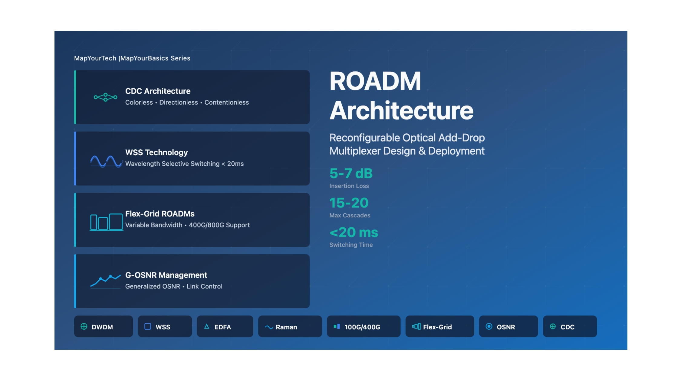
A Reconfigurable Optical Add-Drop Multiplexer (ROADM) is a critical component in modern DWDM networks that provides the flexibility to dynamically add, drop, or pass through individual wavelengths without requiring optical-electrical-optical (OEO) conversion. Unlike fixed add-drop multiplexers (ADMs), ROADMs allow for remote configuration, making them ideal for flex-grid networks where bandwidth can be adjusted as needed.
Why Does ROADM Matter?
The importance of ROADM technology stems from several fundamental needs in modern optical networks:
Flexibility & Dynamic Wavelength Management
ROADMs provide the ability to add or drop specific wavelengths at any node in the network without disrupting other wavelengths. This flexibility is vital for building dynamic, multi-service, and scalable networks that can adapt to changing traffic patterns in real-time.
Cost Efficiency & Power Reduction
ROADMs eliminate the need for electrical conversion at every switching point, reducing power consumption and equipment costs in long-haul or metro networks. This translates to significant OPEX and CAPEX savings for network operators.
Network Resilience & Protection
ROADM-based networks support automatic traffic rerouting in the event of fiber cuts or node failures. Protection switching times of less than 50ms ensure service continuity for critical applications, with support for 1+1 protection, ring protection, and mesh restoration schemes.
When Does ROADM Technology Matter Most?
ROADM architecture becomes critical in several scenarios:
- High-capacity backbone networks requiring dynamic bandwidth allocation
- Metro networks with frequent service provisioning and deprovisioning
- Data center interconnects needing flexible capacity management
- 5G backhaul networks requiring low-latency and high-bandwidth links
- Networks supporting multiple data rates (100G, 200G, 400G, 800G simultaneously)
Mathematical Framework
Power Budget Calculation
The fundamental power budget equation for ROADM networks accounts for all losses and gains along the optical path:
Where losses include:
- Fiber attenuation: 0.2 dB/km at 1550nm
- Connector losses: 0.5 dB per connector
- Splice losses: 0.1 dB per splice
- Mux/Demux losses: 3-5 dB
- ROADM insertion loss: 5-7 dB per ROADM node
ROADM Insertion Loss Calculation
A critical parameter in ROADM network design is the total insertion loss from multiple ROADM nodes:
Parameters:
- α = Fiber attenuation coefficient (dB/km)
- Distance = Total fiber length (km)
- NROADM = Number of ROADM nodes
- ILROADM = Insertion loss per ROADM (typically 5-7 dB)
Generalized OSNR (G-OSNR) Calculation
G-OSNR extends traditional OSNR by considering all noise sources in ROADM networks:
Where:
- Psignal = Total signal power
- Ntotal = Accumulated noise power from all ROADMs, amplifiers, and spans
- Measured in a reference bandwidth of 0.1 nm (12.5 GHz)
Practical Calculation Example
Example: 500 km ROADM Network
Given:
- Distance: 500 km
- Fiber attenuation: 0.25 dB/km
- Number of ROADMs: 5
- ROADM insertion loss: 5 dB each
Calculation:
ROADM Loss = 5 × 5 = 25 dB
Total Attenuation = 125 + 25 = 150 dB
This total attenuation determines the required amplification and OSNR budget for the link.
Key Design Parameters
| Parameter | Typical Value | Design Guideline |
|---|---|---|
| ROADM Insertion Loss | 5-7 dB | Minimize by selecting WSS-based ROADMs |
| Maximum Cascaded ROADMs | 15-20 nodes | Limited by accumulated OSNR degradation |
| Minimum OSNR Requirement | 18-20 dB | Depends on modulation format |
| Channel Power Flatness | ±1 dB | Critical for multi-channel systems |
| Switching Time (MEMS) | <50 ms | Adequate for protection switching |
| Switching Time (WSS) | <20 ms | Faster protection and provisioning |
Types & Components
Evolution of ROADM Technologies
1. Fixed-Grid ROADMs (Generation 1)
Technology: The first generation operated on a fixed-grid architecture with wavelengths constrained to predefined channel spacings (typically 50 GHz or 100 GHz).
Limitations: Limited flexibility, could not accommodate higher-capacity channels like 400G or 1T which require broader bandwidth. Static wavelength routing for 10G or 40G signals only.
Use Case: Early DWDM metro networks with static traffic patterns.
2. Dynamic ROADMs with WSS (Generation 2)
Technology: Introduction of Wavelength Selective Switch (WSS) marked a significant advancement, allowing dynamic switching of wavelengths with flexible routing.
Advantages: Enables flexible routing of any wavelength to any direction, supports mesh networking, reduces manual intervention, switching time <20ms.
Use Case: Long-haul networks requiring real-time routing changes based on traffic patterns.
3. CDC ROADMs (Generation 3)
Technology: Colorless, Directionless, and Contentionless architecture provides maximum flexibility.
Key Features:
- Colorless: Any wavelength can be added/dropped at any port
- Directionless: Traffic can flow in any direction without physical reconnections
- Contentionless: Same wavelength can be routed through multiple paths without interference
Use Case: Nationwide optical backbones requiring full routing flexibility for 100G and 400G channels.
4. Flex-Grid ROADMs (Generation 4)
Technology: Variable bandwidth allocation per channel instead of fixed 50/100 GHz spacing. Channels occupy only the spectrum they require.
Advantages: Efficient spectrum use, supports 400G, 800G, 1T channels, enables seamless upgrades without hardware changes.
Use Case: High-capacity metro networks with mixed data rates (100G, 200G, 400G coexisting).
Component Breakdown
| Component | Function | Key Specifications |
|---|---|---|
| Wavelength Selective Switch (WSS) | Routes signals between fibers according to wavelength using "disperse and switch" configuration | Switching time: <20ms Insertion loss: 5-7 dB Port count: 1×9 to 1×20 typical |
| Optical Channel Monitor (OCM) | Monitors channel power levels at ROADM output | Accuracy: ±0.5 dB Measurement range: -40 to +10 dBm |
| Variable Optical Attenuator (VOA) | Controls individual channel power levels | Attenuation range: 0-30 dB Response time: <10ms |
| Optical Amplifier (EDFA/Raman) | Compensates for insertion loss and fiber attenuation | Gain: 15-25 dB Noise Figure: 4-6 dB |
| Demultiplexer/Multiplexer | Separates/combines wavelength channels | Insertion loss: 3-5 dB Isolation: >30 dB |
Comparison of ROADM Types
| Feature | Fixed-Grid | WSS-Based | CDC | Flex-Grid |
|---|---|---|---|---|
| Flexibility | Low | Medium | High | Very High |
| Wavelength Blocking | Possible | Possible | None | None |
| Spectrum Efficiency | Medium | Medium | High | Very High |
| Supported Data Rates | 10G, 40G | Up to 100G | Up to 400G | 400G, 800G, 1T+ |
| Initial Cost | Low | Medium | High | Very High |
| Operational Complexity | Low | Medium | Medium-High | High |
| Future-Proofing | Poor | Good | Excellent | Excellent |
Effects & Impacts
System-Level Effects of ROADM Deployment
1. Insertion Loss Impact
Effect: Each ROADM node introduces 5-7 dB of insertion loss due to optical switch complexity.
System Impact: Accumulated loss degrades OSNR and limits the number of cascaded ROADMs (typically 15-20 maximum).
Mitigation: Strategic amplifier placement and careful power budget management required.
2. OSNR Degradation
Effect: Each ROADM and amplifier adds noise through ASE (Amplified Spontaneous Emission).
System Impact: Cumulative OSNR degradation limits transmission distance and data rate capacity.
Quantitative Impact: In a 5-ROADM network, OSNR can degrade from 25 dB to 15 dB, potentially requiring higher-power transmitters or better modulation formats.
3. Chromatic Dispersion Accumulation
Effect: Longer paths through multiple ROADM nodes accumulate chromatic dispersion.
System Impact: Limits maximum transmission distance for high-speed channels (200G+).
Threshold: Maximum differential group delay typically 7.5 ps for 40G systems, 2.5 ps for higher rates.
Performance Implications by Modulation Format
| Modulation Format | Required OSNR | Max ROADM Cascades | Typical Reach | Impact Severity |
|---|---|---|---|---|
| QPSK | 13-15 dB | 15-20 | 2000+ km | Low |
| 16-QAM | 21-23 dB | 10-15 | 1000-1500 km | Medium |
| 64-QAM | 27-30 dB | 5-10 | 500-800 km | High |
Tolerance Levels and Thresholds
Critical Performance Thresholds
- Minimum OSNR: 18-20 dB for error-free operation with standard FEC
- Maximum Span Length: 80-120 km without amplification
- Channel Power Flatness: Must maintain ±1 dB across all channels
- Maximum Cascaded ROADMs: 15-20 nodes before regeneration required
- Protection Switching Time: <50ms for network resilience
Impact Severity Classifications
Mitigation Strategies Overview
OSNR Management Strategies
- Use hybrid EDFA+Raman amplification to reduce effective noise figure
- Implement dynamic channel power equalization using VOAs
- Select lower-loss WSS components when available
- Consider regeneration after 10-15 ROADM cascades for high-order modulation
Dispersion Management
- Use NZDSF fiber for long-haul ROADM networks
- Implement electronic dispersion compensation in coherent receivers
- Monitor accumulated dispersion across the path
- Limit path lengths for higher modulation formats
Techniques & Solutions
Implementation Methods
1. MEMS-Based Switching
Technology: Micro-Electro-Mechanical Systems use tiny mirrors to redirect light paths.
Advantages:
- Low insertion loss (3-5 dB)
- Low wavelength dependency
- Excellent port-to-port uniformity
- High reliability
Disadvantages:
- Slower switching speed (<50ms)
- Mechanical wear over time
- Sensitivity to vibration
- Higher cost for large port counts
Best Use Case: Long-haul networks where switching speed is less critical than insertion loss.
2. WSS-Based Switching
Technology: Wavelength Selective Switches use liquid crystal or LCoS technology for wavelength-specific routing.
Advantages:
- Fast switching (<20ms)
- Per-wavelength control
- Dynamic channel equalization
- Supports flex-grid architectures
- No moving parts
Disadvantages:
- Higher insertion loss (5-7 dB)
- Wavelength-dependent loss
- More complex control systems
- Higher power consumption
Best Use Case: Metro and regional networks requiring frequent reconfiguration and mixed data rates.
Technical Approaches Comparison
| Approach | Switching Speed | Insertion Loss | Scalability | Cost | Recommended For |
|---|---|---|---|---|---|
| MEMS-based ROADM | <50ms | 3-5 dB | Good | Medium | Long-haul, stable networks |
| WSS-based ROADM | <20ms | 5-7 dB | Excellent | High | Metro, dynamic networks |
| Fixed ROADM | Manual | 4-6 dB | Limited | Low | Static networks, access |
| CDC ROADM | <20ms | 6-8 dB | Excellent | Very High | Large backbone networks |
Protection Scheme Implementation
1+1 Protection
Method: Working and protection paths both carry traffic simultaneously. Receiver selects best signal.
Advantages: Fastest protection switching (<1ms), no traffic loss during failure
Disadvantages: 100% capacity overhead, requires dual transponders
Implementation: Use Y-cable protection at endpoints with automatic receiver switching
1:1 Protection
Method: Protection path on standby, switches when failure detected on working path.
Advantages: Protection capacity can be shared, lower initial cost
Disadvantages: Switching time <50ms, brief traffic interruption possible
Implementation: ROADM automatically switches to protection fiber upon detecting failure
Ring Protection
Method: Traffic can flow bidirectionally around ring, automatically reroutes on failure.
Advantages: Self-healing, efficient use of capacity, suitable for metro networks
Disadvantages: Requires coordinated node management, complexity increases with size
Implementation: ROADM nodes configured in ring topology with automatic protection switching
Best Practices & Recommendations
Design Best Practices
- Power Budget: Always maintain 3-6 dB margin in power budget calculations
- OSNR Monitoring: Implement continuous OSNR monitoring at all ROADM outputs
- Channel Equalization: Use automatic channel power equalization to maintain ±1 dB flatness
- Amplifier Placement: Position amplifiers to compensate for ROADM insertion loss
- Spare Capacity: Design for 20-30% future capacity growth
- Documentation: Maintain detailed records of all ROADM configurations and paths
Operational Best Practices
- Regular Testing: Perform quarterly OSNR and BER measurements
- Proactive Monitoring: Set threshold alarms for OSNR degradation
- Change Management: Implement rigorous change control for ROADM reconfigurations
- Software Updates: Keep ROADM management software current
- Backup Paths: Always configure protection paths for critical services
Real-World Application Scenarios
Scenario 1: Metro Network Deployment
Challenge: Frequent service additions/deletions in metropolitan area
Solution: WSS-based CDC ROADM with flex-grid support
Result: 80% reduction in service provisioning time, 40% OPEX savings
Scenario 2: Long-Haul Backbone
Challenge: 2000 km link with 20 ROADM nodes, OSNR management critical
Solution: Hybrid EDFA+Raman amplification with low-loss MEMS ROADMs
Result: Maintained 20 dB OSNR for 100G QPSK transmission
Scenario 3: Data Center Interconnect
Challenge: Dynamic capacity allocation between multiple data centers
Solution: CDC ROADM with automated bandwidth-on-demand provisioning
Result: Sub-hour service activation, improved resource utilization
Design Guidelines & Methodology
Step-by-Step Design Process
Phase 1: Requirements Analysis
- Traffic Forecast: Analyze current and projected traffic demands (5-year horizon)
- Service Requirements: Identify data rates needed (10G, 100G, 400G, etc.)
- Geographic Coverage: Map node locations and distances
- Protection Requirements: Define availability targets (99.99%, 99.999%, etc.)
- Budget Constraints: Establish CAPEX and OPEX limits
Phase 2: Network Topology Design
- Topology Selection: Ring, mesh, or hybrid based on geography and protection needs
- ROADM Node Placement: Strategic positioning to minimize hop count
- Fiber Routes: Plan diverse routing for protection
- Degree Planning: Determine 2-degree, 4-degree, or higher degree nodes
Phase 3: Link Budget Calculation
- Fiber Loss: Calculate total fiber attenuation (distance × 0.2-0.25 dB/km)
- Component Loss: Sum all connector, splice, mux/demux losses
- ROADM Loss: Account for insertion loss per node (5-7 dB each)
- Amplifier Gain: Determine required gain to compensate losses
- Margin: Add 3-6 dB safety margin
Phase 4: OSNR Budget Analysis
- Calculate G-OSNR: For each path through network
- Verify Requirements: Ensure OSNR meets modulation format needs
- Identify Bottlenecks: Find paths with marginal OSNR
- Optimize: Adjust amplifier placement or consider regeneration
Decision Framework
IF Static traffic pattern + Cost-sensitive:
→ Fixed-Grid ROADM
ELSE IF Dynamic traffic + Metro network + <500km:
→ WSS-based ROADM
ELSE IF High capacity + Multiple data rates + Frequent changes:
→ CDC ROADM
ELSE IF Future-proof + 400G/800G support + Spectrum efficiency critical:
→ Flex-Grid ROADM
Practical Design Example
Example: 400km Metro Ring Network
Requirements:
- 6 ROADM nodes in ring topology
- Support 40 channels at 100G each (4 Tbps total)
- 50ms protection switching requirement
- Future expansion to 400G channels
Design Decisions:
- ROADM Type: CDC with WSS technology
- Justification: Meets switching time, supports future 400G
- Fiber Type: NZDSF (G.655)
- Justification: Balances dispersion and nonlinear effects
- Amplifier Strategy: EDFA at each ROADM node
- Placement: Pre-amp before ROADM, booster after
Calculations:
Fiber loss per span = 67 km × 0.25 dB/km = 16.75 dB
ROADM insertion loss = 6 dB
Other losses (connectors, mux) = 3 dB
Total loss per span = 25.75 dB
Required amplifier gain = 25.75 dB + 3 dB margin = 28.75 dB
Use: Pre-amp (10 dB) + Booster (20 dB) = 30 dB total
OSNR Verification:
Number of amplifier stages = 12 (2 per ROADM × 6 nodes)
Input power = 0 dBm
Using 58+ formula:
OSNR ≈ 58 + Pout - (L + NF + 10log(N-1))
OSNR ≈ 58 + 0 - (25.75 + 5 + 10.8) = 16.45 dB
For 100G QPSK: Requires ~13-15 dB → PASS with margin
Design Checklist
| Design Element | Checkpoint | Target Value |
|---|---|---|
| Link Budget | Power margin adequate? | ≥3 dB margin |
| OSNR Budget | Meets modulation requirements? | ≥18 dB for most formats |
| Dispersion | Within tolerance? | <7.5 ps for 40G, <2.5 ps for higher |
| ROADM Cascades | Number of nodes reasonable? | ≤15 without regeneration |
| Channel Power | Power flatness acceptable? | ±1 dB across all channels |
| Protection | Switching time meets SLA? | <50ms typical |
| Scalability | Growth capacity planned? | 20-30% headroom |
Common Pitfalls to Avoid
Top Design Mistakes
- Insufficient Margin: Failing to include adequate safety margin (minimum 3 dB)
- Ignoring Cascaded OSNR: Not properly calculating accumulated noise through multiple ROADMs
- Power Budget Errors: Forgetting to account for all connectors, splices, and component losses
- Wrong ROADM Type: Selecting technology that doesn't match operational requirements
- No Protection: Deploying without adequate protection schemes for critical services
- Poor Amplifier Placement: Incorrect amplifier locations leading to suboptimal OSNR
- Ignoring Nonlinearities: Not considering FWM, XPM effects in fully-loaded systems
- Future Growth: Not planning for capacity expansion and technology migration
- Documentation: Poor documentation of ROADM configurations and optical paths
Interactive Simulators
Practical Applications & Case Studies
Real-World Deployment Scenarios
Case Study 1: Financial Services Data Center Interconnect
Challenge: A large financial institution needed to increase inter-data-center bandwidth during market hours while maintaining sub-millisecond latency and 99.999% availability.
Initial Situation:
- Static 100G connections between 4 data centers
- Traffic congestion during peak trading hours (9am-4pm)
- Manual provisioning taking 2-3 weeks
- Limited ability to respond to market volatility
Solution Approach:
- Deployed CDC-ROADM nodes at each data center location
- Implemented dynamic bandwidth allocation using WSS technology
- Configured 1+1 protection for all critical paths
- Integrated with SDN controller for automated provisioning
Implementation Details:
- Used 4-degree CDC ROADMs with flex-grid capability
- Deployed hybrid EDFA+Raman amplification
- Maximum distance between sites: 150 km
- Average OSNR maintained at 22 dB
Results & Benefits:
- ✓ Provisioned additional 100G channels in under 1 hour
- ✓ Reduced bandwidth costs by 35% through dynamic allocation
- ✓ Achieved 99.9995% availability with protection switching <50ms
- ✓ Enabled real-time capacity adjustment based on trading volume
- ✓ ROI achieved in 18 months
Case Study 2: Long-Haul Backbone Network Upgrade
Challenge: A national carrier needed to upgrade a 2000 km backbone network to support 100G and prepare for 400G while maintaining existing 10G/40G services.
Initial Situation:
- 20 fixed ROADM nodes with limited reconfiguration capability
- Approaching 80% capacity utilization
- Growing demand for high-capacity services
- Complex manual reconfiguration process
Solution Approach:
- Phased migration to flex-grid WSS-based ROADMs
- Deployed coherent 100G transponders with adaptive modulation
- Implemented distributed Raman amplification
- Upgraded network management system for automated control
Implementation Details:
- Replaced 5 critical nodes in phase 1 (metro aggregation points)
- Used low-loss WSS modules (insertion loss 5.5 dB)
- Maintained service during upgrade using protection paths
- G-OSNR calculations verified at each phase
Results & Benefits:
- ✓ Increased network capacity from 800 Gbps to 4 Tbps
- ✓ Reduced service provisioning time from weeks to hours
- ✓ Enabled dynamic routing around failures
- ✓ Maintained OSNR >20 dB across all paths
- ✓ 40% reduction in OPEX through automation
- ✓ Ready for 400G migration without hardware replacement
Case Study 3: 5G Mobile Backhaul Network
Challenge: A mobile operator needed to deploy 5G backhaul with ultra-low latency (<5ms) and dynamic bandwidth allocation to support varying traffic patterns across regions.
Initial Situation:
- 4G backhaul insufficient for 5G data rates
- Static bandwidth allocation inefficient for 5G traffic
- Need for low-latency optical switching
- Budget constraints limiting fiber deployment
Solution Approach:
- Deployed metro ROADM network with 2-degree and 4-degree nodes
- Implemented traffic-aware dynamic bandwidth allocation
- Used existing fiber infrastructure with DWDM overlay
- Integrated with 5G core network orchestration
Implementation Details:
- 40 ROADM nodes across metropolitan area
- Average fiber distance: 15-30 km per span
- WSS switching time: <20ms
- 40 wavelength channels supporting mixed 25G/100G/400G
Results & Benefits:
- ✓ Achieved average latency of 2.5ms across network
- ✓ Dynamic bandwidth allocation improved efficiency by 45%
- ✓ Supported peak data rates during events (concerts, sports)
- ✓ Reduced backhaul costs per Gbps by 60%
- ✓ Network scales to support future 5G-Advanced requirements
Troubleshooting Guide
| Issue | Symptoms | Likely Causes | Solutions |
|---|---|---|---|
| Low OSNR | High BER, service degradation, alarm thresholds exceeded | Excessive amplifier noise, too many cascaded ROADMs, fiber loss higher than expected | Check amplifier NF, verify fiber condition, add regeneration, optimize amplifier placement |
| Channel Power Imbalance | Some channels good, others poor; uneven OSNR across spectrum | WSS misconfiguration, amplifier gain tilt, failed VOA | Recalibrate WSS, adjust VOA settings, enable automatic gain control, check amplifier equalization |
| Switching Failures | Protection path not activating, service interruptions during reconfiguration | WSS calibration drift, control plane issues, fiber breaks not detected | Recalibrate WSS, verify monitoring systems, check APS protocol configuration, test protection paths |
| High Insertion Loss | Lower than expected received power, reduced reach | Dirty connectors, WSS degradation, accumulated component loss | Clean all connectors, verify component specifications, measure insertion loss at each element |
| Crosstalk | Interference between channels, ghost signals | Insufficient channel isolation, WSS filter issues, nonlinear effects | Increase channel spacing, recalibrate WSS filters, reduce channel power, check for FWM |
| Dispersion Issues | Pulse broadening, reduced reach for high-speed channels | Accumulated chromatic dispersion, PMD, long path through network | Enable electronic dispersion compensation, verify fiber type, consider regeneration, check coherent receiver DSP |
Quick Reference Tables
ROADM Selection Guide
| Application | Recommended ROADM | Key Features | Typical Cost Range |
|---|---|---|---|
| Metro Access (<100km) | Fixed-Grid or WSS | Simple, cost-effective, adequate flexibility | $ |
| Regional Network (100-500km) | WSS-Based ROADM | Dynamic routing, good performance | $ |
| Long-Haul Backbone (>500km) | CDC ROADM | Maximum flexibility, high capacity | $$ |
| Data Center Interconnect | CDC or Flex-Grid | Dynamic bandwidth, multi-rate support | $$ |
| 5G Backhaul | WSS or CDC | Low latency, dynamic allocation | $-$$ |
Performance Optimization Tips
| Parameter | Target Value | Optimization Technique |
|---|---|---|
| OSNR | >20 dB | Use Raman amplification, reduce cascades, optimize launch power |
| Insertion Loss | <6 dB per ROADM | Select low-loss WSS, maintain clean connectors, minimize splices |
| Channel Flatness | ±0.5 dB | Enable automatic gain control, use VOA arrays, regular calibration |
| Switching Time | <20 ms | Use WSS technology, optimize control plane, pre-configure paths |
| Spectral Efficiency | >3 b/s/Hz | Flex-grid deployment, higher-order modulation, tight channel spacing |
Professional Recommendations
Industry Best Practices
- Start with Requirements: Thoroughly analyze traffic patterns and growth projections before selecting ROADM technology
- Future-Proof Design: Choose technology that supports next-generation data rates (400G, 800G)
- Monitor Continuously: Implement comprehensive performance monitoring at all ROADM nodes
- Document Everything: Maintain detailed records of configurations, optical paths, and power budgets
- Test Protection Paths: Regularly verify that protection switching works as designed
- Plan for Growth: Design with 20-30% spare capacity for future expansion
- Automate Where Possible: Leverage SDN and automation for provisioning and optimization
- Train Operations Staff: Ensure team understands ROADM technology and troubleshooting procedures
- Vendor Selection: Consider total cost of ownership, not just initial equipment cost
- Regular Maintenance: Schedule periodic cleaning, calibration, and testing

Optical Communications & Network Automation Expert | Author of 3 Books for Optical Engineers | Founder, MapYourTech
Optical networking engineer with nearly two decades of experience across DWDM, OTN, coherent optics, submarine systems, and cloud infrastructure. Founder of MapYourTech. Read full bio →
Follow on LinkedIn