
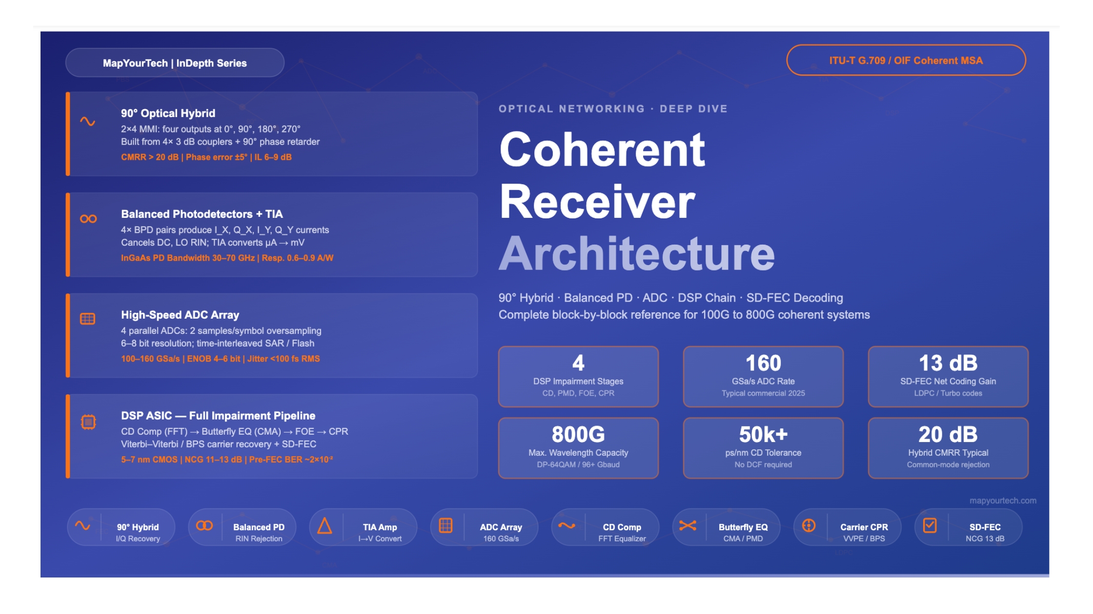

Coherent Receiver Architecture:
Quick-Reference Block Diagram
1. Introduction
The coherent receiver as the cornerstone of high-capacity optical transport
The coherent optical receiver is the defining technological achievement that has enabled modern high-capacity optical transport networks. By recovering both the amplitude and phase of the received optical field — in both polarization tributaries simultaneously — the coherent receiver unlocks advanced modulation formats such as Dual-Polarization Quadrature Phase-Shift Keying (DP-QPSK), DP-16QAM, DP-64QAM, and beyond. This capability transforms a single wavelength from a simple intensity-modulated channel into a multi-dimensional information carrier capable of transporting 100 Gbps, 400 Gbps, and now 800 Gbps in commercial deployments.
The contrast with legacy intensity-modulation direct-detection (IM-DD) receivers is fundamental. A direct-detection receiver discards the phase information entirely, capturing only the envelope of the optical power. The result is a severe constraint: only amplitude-keyed modulation formats are accessible, spectral efficiency is limited, and dispersion tolerance without optical compensation modules is poor. The coherent receiver eliminates all three limitations. Phase, amplitude, and both polarization states are preserved through the detection process. Chromatic dispersion (CD), polarization mode dispersion (PMD), and even carrier phase noise — impairments that dominated system design in the IM-DD era — become purely digital compensation problems.
From a system architecture perspective, the coherent receiver is composed of several tightly coupled functional stages. At the optical level, a polarization beam splitter (PBS) separates the incoming signal into two orthogonal polarization tributaries, which are mixed with a tunable local oscillator (LO) laser through a pair of 90-degree optical hybrids. The resulting four complex-field projections — IX, QX, IY, QY — are converted to electrical currents by balanced photodetector pairs, amplified by transimpedance amplifiers (TIAs), and then digitized by four analog-to-digital converters (ADCs). The digital samples flow into a multi-stage DSP pipeline that sequentially compensates every major impairment and ultimately delivers decoded data to the framer or host system.
This article serves as a complete technical reference for the coherent receiver block diagram, covering each stage with sufficient depth for engineers working on system design, procurement evaluation, or DSP algorithm development. Formulas are provided where they illuminate the signal processing principles, and practical parameter ranges reflect commercial 100G–800G deployment experience.
2. Historical Evolution
From concept to commercial deployment: the coherent receiver timeline
Coherent optical detection was studied extensively in the 1980s and early 1990s, primarily for its receiver sensitivity advantage. In homodyne and heterodyne detection, the local oscillator power amplifies the signal-photocurrent term, improving sensitivity by approximately 15–20 dB compared to direct-detection receivers. Laboratory demonstrations of coherent FSK, PSK, and CPFSK systems were reported during this period, but the technology faced a critical obstacle: maintaining phase synchronization between the LO and the transmitted carrier in a deployed fiber plant required phase-locked loops whose practical implementation was extremely complex at optical frequencies.
The advent of the erbium-doped fiber amplifier (EDFA) in the early 1990s shifted the industry focus back to IM-DD systems with optical amplification. EDFAs compensated for fiber loss without O/E conversion, and combined with dispersion-shifted fiber and later dispersion-compensating fiber, the IM-DD paradigm expanded to 10 Gbps and then 40 Gbps per wavelength. Throughout this period, coherent detection remained a research topic rather than a commercial reality.
The transformation occurred in the mid-2000s. Two insights converged: first, it was recognized that carrier phase noise could be compensated in the digital domain using DSP algorithms rather than analog phase-locked loops; second, CMOS ASIC technology had progressed to the point where DSPs capable of 56–64 GSamples/s throughput were manufacturable at acceptable power and cost. Savory et al. demonstrated digital equalization of 40 Gbit/s per wavelength over 2480 km of standard fiber in 2006 without optical dispersion compensation, a result that conclusively proved the viability of the DSP-enabled coherent approach. This was followed by rapid industry standardization around DP-QPSK at 112 Gbps gross line rate, which became the first commercially deployed coherent format and is defined in standards such as ITU-T G.709 and OIF-100G-LR-MSA.
By 2010, 100G DP-QPSK coherent transponders were shipping commercially. The subsequent decade saw a systematic progression: 200G DP-16QAM, then 400G with probabilistic shaping, then 800G targeting data center interconnect. Each generation demanded improvements in ADC resolution and sampling rate, DSP power efficiency, laser linewidth, and optical hybrid performance. Photonic integrated circuit (PIC) technology — initially implemented in Indium Phosphide (InP) and then in silicon photonics — further reduced the form factor and cost, enabling pluggable coherent modules in CFP2, QSFP-DD, and OSFP form factors.
Evolution Summary
- 1980s–early 1990s: Coherent detection studied for sensitivity, but impractical due to phase-locking complexity
- 1990s: EDFA enabled IM-DD dominance; coherent relegated to research
- 2006: DSP-enabled coherent demonstrated — phase tracking moved to digital domain
- 2010: First commercial 100G DP-QPSK coherent deployments
- 2015–2025: Rapid progression through 200G, 400G, 800G with PIC integration
Read the Full Analysis with Premium
The remaining 89% of this article — the design numbers, trade-offs and field guidance — is part of MapYourTech Premium, along with the full premium library, courses and professional tools.



Course Title
Course description and key highlights
Course Content
Course Details
Celebrating 1,000+ LinkedIn posts
3 hours of Premium Pro, free
The full Premium Pro library, unlocked with one click. The clock starts the moment you check out and runs for 3 full hours - pick a time when you can make the most of it.
- Courses
- Interview preparation content
- Career development posts
- Simulators
- Calculators
- Market research
No card, nothing to cancel. One pass per person. Sign in or create a free account at checkout.
Follow MapYourTech on LinkedIn for regular updates and future promos.
New articles, tool releases and member offers, posted as they go live.
Follow MapYourTech on LinkedIn
Enjoying MapYourTech? Follow us on LinkedIn. One click and this stops appearing.
- New technical articles and tool releases, posted as they go live
- Course launches and member offers before they reach the site
- Standards and industry updates worth an optical engineer's time
New articles, tool releases and member offers, posted as they go live.