
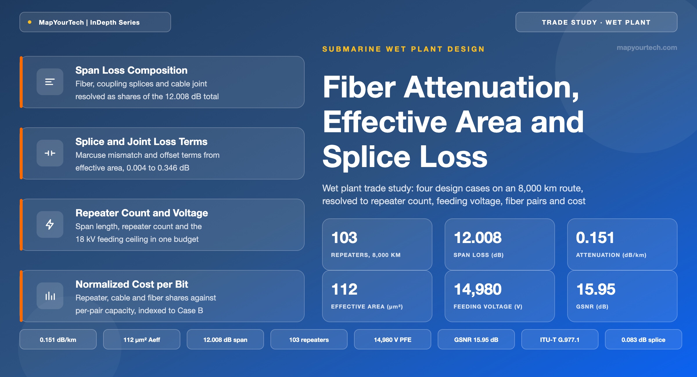
Fiber Attenuation, Effective Area and Splice Loss Trade Study for Wet Plant
How each fiber parameter moves repeater count, system voltage and cost per bit on a fixed route, and what a single fiber type per span returns in deployment and repair.
Loss is measured in the field, not read from a datasheet.
What You Will Learn
- Define span loss and repeater section from first principles and place every contributing element, using the 12.008 dB reference budget of Figure 1.
- Convert effective area to mode field diameter and back, and check the result against the 9.5–10.5 µm and 11.5–15.0 µm nominal ranges of ITU-T G.654.C and G.654.D.
- Quantify the mode-field mismatch penalty at a dissimilar splice with the Marcuse expression, from 0.005 dB at 80 µm² to 0.346 dB at 150 µm².
- Derive why repeater spacing scales as 1/α and powering-constrained cable capacity as 1/α², and apply both to a 0.158 → 0.146 dB/km change.
- Build the power feeding voltage stack for an 8,000 km route and read off the 14,800–15,280 V band the three design cases produce.
- Convert saved voltage into line current and fiber pairs, and see 0.012 dB/km return 4.9% more current under an 18 kV ceiling.
- Anchor the repair budget on the ITU-T G.977.1 guidance of one deep-water repair per 1,000 km and one shallow-water repair per 15 km.
- Select a fiber for a given route from the four-case design analysis of Section 9, and state what a single fiber type per span returns at repair time.
1. Introduction
A wet plant contract fixes three numbers before anything is manufactured: how many repeaters sit on the seabed, what voltage the power feeding equipment must hold at each shore end, and how many fiber pairs the cable carries. All three follow from the cabled attenuation coefficient, the effective area and the joint loss of the fiber that goes into the cable, and all three are settled years before the first transponder is chosen. The fiber decision is therefore the earliest irreversible decision in the system, and it is taken on parameters that differ between candidates by a few thousandths of a decibel per kilometer and a few tens of square micrometers.
Those differences look small on a datasheet and are not small in a system. Commercially available submarine fibers span roughly 0.144 to 0.158 dB/km at 1550 nm with effective areas from 80 to 153 µm² (vendor-published envelope, major submarine fiber suppliers). Across that range the powering-constrained capacity of a fixed route changes by a factor approaching 1.2, the optimum repeater spacing changes by 8%, and the number of repeaters the owner buys and the power feeding equipment must energize changes by several units on a transoceanic length. The trade is not between a good fiber and a bad one. It is between three fibers that each win a different term of the same budget.
This article works the trade for one fixed route: 8,000 km, point-to-point, C-band, space division multiplexing design practice, single fiber type per span. It sets up the loss budget from first principles, derives the mode-field mismatch penalty that large effective area imposes at every dissimilar splice, propagates both into repeater count and power feeding voltage, converts spare voltage into line current and fiber pairs, and closes with a normalized cost-per-bit comparison and the operational return from a single fiber type. Where a figure comes from a Recommendation it is labeled standard-specified; where it is a manufacturer envelope it is labeled a vendor-published figure; where it is a physical bound it is labeled a theoretical limit; and where it is a value chosen for this trade study it is labeled a design value so that a reader can substitute their own.
The scope stops at the wet plant. Terminal equipment, modulation format selection and the submarine line terminal equipment upgrade path are treated only where they set a boundary condition on the fiber choice. The terminal side of the same system is carried in the open cable, generalized OSNR and power-constrained transmission treatment, and the boundary between the two domains is drawn in wet plant versus dry plant equipment.
2. Span Loss and Repeater Section Definitions
Span loss is the total optical attenuation, in decibels at a stated reference frequency, between the output of one submarine repeater and the input of the next. It aggregates the cabled fiber attenuation over the span length with every discrete loss element in that length: repeater coupling splices, cable joint splices, and the insertion loss of any gain or tilt equalizer housed within the section. Span loss sets the gain each repeater must supply.
2.1 Distinctions From Adjacent Quantities
Four quantities are routinely conflated in wet plant discussion, and every one of them is a different number in the ITU-T G.977.1 key parameter table.
Span length against repeater spacing. Span length is the cable distance between consecutive repeaters and is what multiplies the attenuation coefficient. Repeater spacing is the same distance viewed as a design choice, and the two diverge after a repair inserts cable into an existing section.
Span loss against fiber attenuation. Fiber attenuation is a per-kilometer coefficient of the cabled fiber. Span loss is the total decibel figure for the section, including splices. A design that reports only the coefficient has not stated the repeater gain requirement.
Uncabled attenuation against cabled attenuation. The datasheet figure is measured on fiber on a shipping spool. The cabled figure includes any microbending contribution introduced by the cable structure, and it is the cabled figure that closes the budget.
Read the Full Analysis with Premium
The remaining 89% of this article — the design numbers, trade-offs and field guidance — is part of MapYourTech Premium, along with the full premium library, courses and professional tools.
You May Also Like
-
Free
-
August 22, 2026
-
Premium
-
August 22, 2026
-
Premium
-
August 22, 2026