
Introduction to Link Budget Analysis
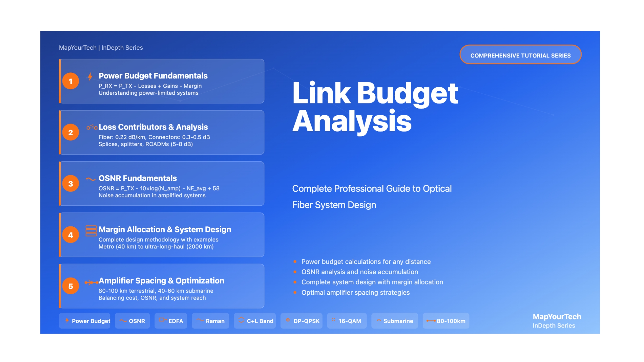
Master the fundamentals of optical power budgets and understand why link budget analysis is critical for designing reliable optical fiber communication systems
Why Link Budget Analysis Matters
In optical fiber communication systems, link budget analysis serves as the foundation for network design and planning. It's the systematic accounting of all power gains and losses throughout an optical transmission path, from the transmitter to the receiver. Think of it as the financial budget for your optical link—except instead of tracking dollars, you're tracking optical power measured in decibels (dB).
Whether you're designing a 10 km metropolitan network or a 1,000 km long-haul system, link budget analysis answers the critical question: Will my optical signal have enough power to reach the receiver and maintain acceptable performance?
Real-World Impact
Global IP traffic is expected to reach 396 exabytes per month by 2025, and network downtime can cost enterprises up to $5,600 per minute. Proper link budget analysis during the design phase prevents costly failures, reduces operational expenses, and ensures reliable high-speed connectivity. A single miscalculation can mean the difference between a functioning 100G link and complete signal loss.
What is Link Budget?
Link budget is a comprehensive calculation that accounts for all factors affecting optical signal power as it travels from transmitter to receiver. It ensures that the received optical power is sufficient for the receiver to detect and decode the signal correctly, maintaining an acceptable bit error rate (BER).
At its core, link budget analysis involves three fundamental components:
- Power Sources (Gains): Transmitter output power, optical amplifier gains
- Power Losses: Fiber attenuation, connector losses, splice losses, component insertion losses
- Power Requirements: Receiver sensitivity, system margin for reliability
Core Concepts: The Power Budget Equation
The fundamental link budget equation provides the framework for all optical link calculations. In its simplest form, it states that the received power must equal the transmitted power minus all losses plus any gains:
Basic Link Budget Equation
PRX = PTX - Total Losses + Total Gains - System Margin
Where:
- PRX = Received power at the detector (dBm)
- PTX = Transmitted power from the source (dBm)
- Total Losses = Sum of all power losses in the link (dB)
- Total Gains = Sum of amplifier gains (dB), if applicable
- System Margin = Safety margin for unforeseen losses and aging (dB)
For most systems without optical amplifiers (unamplified links), the equation simplifies to:
Simplified Link Budget (No Amplifiers)
PRX = PTX - (α × L) - ΣLconnectors - ΣLsplices - Lcomponents - M
Where:
- α = Fiber attenuation coefficient (dB/km), typically 0.2-0.25 dB/km at 1550 nm
- L = Fiber length (km)
- ΣLconnectors = Total connector losses (typically 0.1-0.5 dB per connector)
- ΣLsplices = Total splice losses (typically 0.05-0.1 dB per splice)
- Lcomponents = Losses from multiplexers, demultiplexers, filters, etc.
- M = System margin (typically 3-6 dB)
Critical Success Criterion
For a link to function properly, the received power must exceed the receiver sensitivity threshold:
PRX ≥ Receiver Sensitivity
Critical Design Rule
If the calculated received power falls below the receiver sensitivity threshold, the link will not function correctly. This results in high bit error rates (BER), frequent signal dropouts, and potential complete communication failure. Always include adequate system margin (3-6 dB) to account for aging, environmental factors, and unforeseen losses.
Understanding Key Link Budget Parameters
1. Transmitter Output Power (PTX)
The transmitter output power is the optical power launched into the fiber by the optical transmitter or transceiver. This is typically specified in dBm (decibels relative to 1 milliwatt) and varies based on the transceiver type and data rate.
| Transceiver Type | Typical TX Power | Application |
|---|---|---|
| SFP (1G) | -3 to 0 dBm | Short reach metro/access |
| SFP+ (10G) | -1 to +2 dBm | Data center, metro |
| QSFP28 (100G) | -2 to +2 dBm | Data center interconnect |
| CFP2-DCO (100G/200G) | 0 to +5 dBm | Long-haul coherent |
| 400G ZR/ZR+ | 0 to +4 dBm | DCI and metro DWDM |
2. Receiver Sensitivity (PRX,min)
Receiver sensitivity defines the minimum optical power level required at the receiver input to achieve acceptable bit error rate (BER) performance, typically 10-12 or better. This parameter is critical because it sets the lower bound for acceptable received power.
| Data Rate | Modulation | Typical Sensitivity |
|---|---|---|
| 1G | NRZ | -24 to -28 dBm |
| 10G | NRZ | -18 to -24 dBm |
| 25G | NRZ | -14 to -18 dBm |
| 100G | 4×25G NRZ | -12 to -16 dBm |
| 100G | DP-QPSK | -20 to -24 dBm |
| 200G | DP-16QAM | -15 to -18 dBm |
Understanding the Pattern
Notice that receiver sensitivity becomes less sensitive (requires more power) as data rates increase. This is due to reduced signal-to-noise ratio tolerance at higher speeds. Coherent modulation formats (QPSK, 16QAM) typically offer better sensitivity than direct detection schemes at equivalent data rates.
3. Fiber Attenuation (α)
Fiber attenuation represents the optical power loss per unit length of fiber, measured in dB/km. This is typically the largest contributor to total link loss in most optical systems.
| Wavelength | Typical Attenuation | Application |
|---|---|---|
| 850 nm | 2.5-3.5 dB/km | Multimode short reach |
| 1310 nm (O-band) | 0.30-0.35 dB/km | Metro, zero dispersion |
| 1550 nm (C-band) | 0.18-0.22 dB/km | Long-haul, DWDM |
| 1625 nm (L-band) | 0.20-0.25 dB/km | Extended DWDM |
For design purposes, conservative values are typically used:
- 1310 nm: 0.35 dB/km (accounts for aging and splices)
- 1550 nm: 0.25 dB/km (most common for long-haul systems)
4. System Margin (M)
System margin is additional power budget allocated to account for:
- Component aging: Laser power degrades over time (typically 1-2 dB over 15-20 years)
- Environmental factors: Temperature variations affect component performance
- Maintenance activities: Temporary additional losses during repairs
- Unforeseen losses: Fiber bends, contamination, future splices
- Measurement uncertainties: Equipment calibration tolerances
| Application | Typical Margin | Rationale |
|---|---|---|
| Short reach (< 10 km) | 2-3 dB | Minimal aging concerns |
| Metro (10-80 km) | 3-5 dB | Standard design practice |
| Long-haul (> 80 km) | 5-6 dB | Extended service life |
| Submarine cables | 6-8 dB | Difficult/costly repairs |
Hands-On Exercise #1: Simple Point-to-Point Link
Problem Statement
You need to design a 10G optical link between two buildings separated by 50 km. Calculate whether the link is feasible and what margin you have.
Given Parameters
- Distance: 50 km
- Transmitter power: +2 dBm (10G SFP+)
- Receiver sensitivity: -20 dBm
- Fiber attenuation: 0.25 dB/km @ 1550 nm
- Number of connectors: 4 (2 at each end)
- Connector loss: 0.3 dB each
- Number of splices: 2 (intermediate)
- Splice loss: 0.1 dB each
- Required system margin: 3 dB
Step-by-Step Solution
Step 1: Calculate fiber attenuation loss
Fiber Loss = α × L = 0.25 dB/km × 50 km = 12.5 dB
Step 2: Calculate connector losses
Connector Loss = 4 connectors × 0.3 dB = 1.2 dB
Step 3: Calculate splice losses
Splice Loss = 2 splices × 0.1 dB = 0.2 dB
Step 4: Calculate total losses
Total Loss = 12.5 + 1.2 + 0.2 = 13.9 dB
Step 5: Calculate received power
Read the Full Analysis with Premium
The remaining 89% of this article — the design numbers, trade-offs and field guidance — is part of MapYourTech Premium, along with the full premium library, courses and professional tools.