
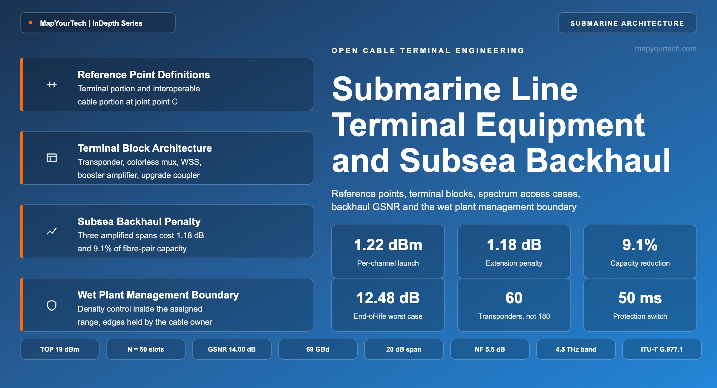
Submarine Line Terminal Equipment and Backhaul Integration
Terminal blocks from transponder to line interface, subsea backhaul with in-line amplifiers and ROADMs, optical multiplex section protection, and the management separation between wet plant control and upgrade equipment.
A network is designed once and operated for twenty years.
What You Will Learn
- Define the terminal portion and the interoperable cable portion from the MPI and IPI reference points of Figure 1, and place the optical coupling junction at joint point C.
- Convert a repeater total output power of 19 dBm across 60 slots into the 1.22 dBm per-channel launch that the coupling junction has to present.
- Compose SNRASE, SNRNLI and SNRGAWBS into GSNR by the inverse-sum and droop product rules, and scale a 17.0 dB OSNR into 9.22 dB at 75 GHz spacing.
- Build the transmit chain of Section 5 block by block, from transponder through colorless multiplexer and wavelength selective switch to the upgrade coupler.
- Select among the three optical cable interface access cases of Table 4, including the spectrum management block that isolates two capacity holders on one fibre pair.
- Quantify a terrestrial extension: three 100 km spans at 20 dB span loss cost 1.18 dB of GSNR and 9.1% of fibre-pair capacity, taking 33.1 Tb/s to 30.1 Tb/s.
- Carry the interoperable cable budget of Table 6 to a 12.48 dB end-of-life worst case and read off the line rate it supports after flooring to 100 Gb/s granularity.
- Set the management boundary of Figure 8 so that a channel turn-up needs one system, not two, while the wet plant domain still enforces the aggregate density.
1. Introduction
A submarine cable landing station holds two pieces of equipment that share one fibre and almost nothing else. On one side of the coupling point sits the wet plant and everything that manages it: repeaters, branching units, power feed equipment and the line monitoring gear that interrogates them, all bought once under a supply contract that assumes a 25-year design life. On the other side sits the terminal that converts client traffic into a modulated optical spectrum, and it will be replaced three or four times inside that same period, because coherent modem generations turn over every three to five years. Submarine line terminal equipment (SLTE) is the name for that second block, and the engineering question this article works through is where exactly the boundary between the two falls, what crosses it, and what happens to the numbers when the terminal moves several hundred kilometres inland.
The boundary matters because it decides who owns which parameter. In a turnkey system the question does not arise: one supplier delivers wet plant and terminal together, and the acceptance test is a bit error rate measured through that supplier's own transponders. In an open cable system the wet plant is delivered without transponders, acceptance is measured in generalized signal-to-noise ratio (GSNR) against a wet-plant-only specification, and the terminal arrives later from whichever supplier wins that separate contract. Every quantity that used to live inside one vendor's design margin becomes a written interface term: the passband edges, the launch power spectral density, the loading rules that apply when a channel fails, and the monitoring access that has to keep working whether or not any traffic is present.
Terminating that spectrum at the landing station is optically cheapest and operationally hardest. Landing stations were sited for cable engineering, not for compute: they sit where the marine route reaches shore, which is rarely where power, floor space and interconnection are available. As of 2026 the constraint that decides the terminating site is power availability rather than fibre, with new hyperscale facilities being commissioned at grid loads that many coastal markets cannot supply, and grid interconnection queues in the largest data centre markets running to several years. The result is a design pattern in which the coupling junction and the wet-plant monitoring stay at the landing station while the transponders sit at a point of presence 100 to 500 km inland, connected by a backhaul chain of in-line amplifiers. That extension is not free, and Section 7 prices it.
Three questions organise what follows. What does the terminal contain, block by block, and which of those blocks belong to the cable owner rather than the capacity holder? What does moving the transponders inland cost in GSNR, in line rate and in equipment count? And where does the management boundary have to sit so that a channel turn-up is one operation in one system rather than a negotiation between two? The scope is repeatered, dispersion-unmanaged, coherent-detected systems with terminal equipment potentially supplied by a different vendor from the wet plant; unrepeatered and festoon systems follow different loading and monitoring rules and are outside it.
2. Terminal Portion and Interoperable Cable Portion Definitions
The terminal portion of a submarine cable system is the part between the client-side system interface in the terminal station and joint point C, where the terminal transmission equipment meets the optical coupling junction. It contains the transponders, the multiplexing and switching photonics, the amplification that sets coupling power, and the management that operates them. Everything on the seaward side of joint point C, including the coupling junction itself, is the interoperable cable portion.
2.1 Adjacent Quantities That Get Conflated
Four distinctions carry most of the confusion, and each is one sentence. The optical coupling junction (OCJ) is the equipment that joins monitoring signals to the traffic spectrum and forwards both into the cable; the optical cable interface (OCI) is the commercial name for the reduced terminal built around that junction on an open cable, and it may contain rather more than the junction alone. The terminal transmission equipment (TTE) is the equipment on the terminal side of joint point C, which on an open cable is the upgrade supplier's kit rather than the wet-plant supplier's. Longitudinal compatibility means both ends of an optical section come from one manufacturer, whereas transverse compatibility means equipment from different manufacturers can be mixed within one section — and what repeatered submarine systems actually offer is the partial case, where all submerged plant comes from one vendor across all fibre pairs while the terminals at either end come from another, with both ends of any single link still matched to each other. And the main path interface pair MPI-SM to MPI-RM bounds the span-loss path through the cable, while the interoperable path interface pair IPI-SM to IPI-RM sits one step further out, on the terminal side of each coupling junction: transverse compatibility is guaranteed before the junction on transmit and after it on receive, so the junction's own loss and coupling behaviour belong to the cable portion rather than to the terminal.
2.2 Units and the Conversion at the Reference Point
The quantity that crosses the reference point is power per channel in dBm, derived from the repeater total output power and the number of loaded slots.
- P — average power per channel at the reference point, in dBm. Typical range for a repeatered C-band system: −3 to +3 dBm.
- TOP — repeater total output power, in dBm, fixed by the submerged amplifier design and unchanged by how the terminal fills the band. Typical range: 15 to 21 dBm.
- N — number of channels or equivalent slots loading the spectrum, dimensionless. A 4.5 THz passband on 75 GHz spacing gives N = 60.
Read the Full Analysis with Premium
The remaining 89% of this article — the design numbers, trade-offs and field guidance — is part of MapYourTech Premium, along with the full premium library, courses and professional tools.
You May Also Like
-
Free
-
August 22, 2026
-
Premium
-
August 22, 2026
-
Premium
-
August 22, 2026