
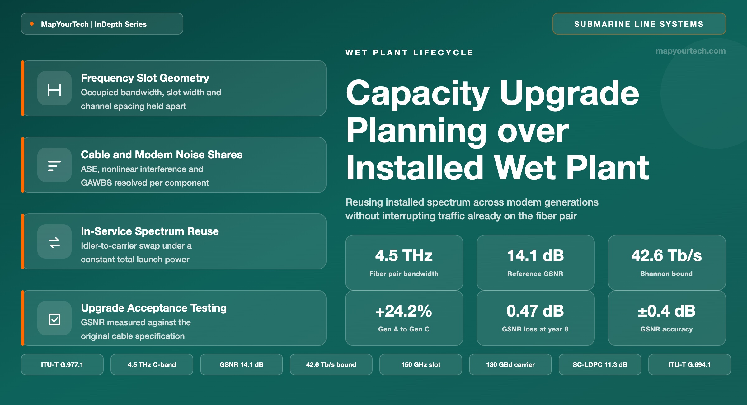
Capacity Upgrade Planning over Installed Wet Plant
An 18-to-24-month modem generation cadence runs against a 25-year wet plant: spectrum reuse, coexistence with channels already in service, and acceptance of an upgrade against the original cable specification.
Fiber is the part of the network that outlives its designers.
What You Will Learn
- Define the frequency slot and its power spectral density envelope, and separate both from occupied bandwidth and channel spacing (Section 2, Figure 1).
- Convert a −15.0 dBm/12.5 GHz density target into the +4.8 dBm total power a 1,200 GHz allocation must present at the interface.
- Quantify achievable capacity from a measured GSNR of 14.1 dB over 4.5 THz, and separate the 42.6 Tb/s theoretical bound from the 27.5 Tb/s a real modem delivers (Section 4).
- Attribute a generation gain to its three sources — modem noise, gap to Shannon, and spectral occupancy — on a wet plant whose GSNR has not moved (Section 6, Table 5).
- Anchor a mid-life measurement to the commissioning baseline using a flat transmit profile rather than an equalized one (Section 6, Figure 6).
- Build a 1:1 idler-to-carrier swap procedure that holds live-channel power to ±0.2 dB across a spectrum reuse step (Section 7, Figure 7).
- Place three 50 GHz legacy slots and one 150 GHz replacement slot on the same 6.25 GHz grid anchored at 193.1 THz (Section 7, Figure 8).
- Select an upgrade path — channel add, parallel line system, or migration — against coupler availability and idler ownership (Section 10, Figure 11).
1. Introduction
A repeatered submarine cable is engineered for a 25-year service life, and the amplifiers, cable and branching units that make up the wet plant are unreachable for that entire period except by a cable ship. The submarine line terminal equipment at each landing station has no such constraint. Vendor-published open-cable guidance places coherent modem technology on an 18-to-24-month generational update cadence, and a separate vendor briefing puts the coherent optical engine technology cycle at four years against the same 25-year cable design life (both vendor claims). Whichever figure a planner uses, the arithmetic is the same: a cable laid today will see somewhere between six and fifteen modem generations pass over it before it is recovered.
That mismatch is the whole subject of upgrade planning. The wet plant delivers a fixed, measurable transmission quality — a generalized signal-to-noise ratio that changes only through aging and repairs — and every capacity gain after commissioning has to be extracted from the terminal. The planner's problem is therefore not "how much more can this cable carry" in the abstract, but three concrete questions. How much spectrum can be freed and reoccupied without disturbing the channels already earning revenue? What does the next modem generation actually buy on a GSNR that has not moved? And against what document does the operator accept the result, given that the original cable specification was written before the modem existed?
1.1 The Two Clocks
Wet plant performance is set at manufacture. Repeater output power, amplifier bandwidth, noise figure, span length and fiber effective area are fixed when the cable ship leaves the factory, and the only post-installation changes are downward: fiber attenuation rises by roughly 0.002 dB/km over 25 years, a deep-water repair inserts about 3 dB of additional span loss, a shallow-water repair about 0.5 dB, and a fraction of repeaters lose a 980 nm pump over the life of the system (all four are design-assumption values used in published end-of-life budget calculations). The aggregate effect on OSNR is small — under 2 dB on the systems modelled in Section 6 — but it is monotonic, and it is the only term in the budget that a terminal upgrade cannot recover.
Terminal performance moves in the other direction and much faster. Each modem generation improves three separable quantities: the equivalent modem noise SNRm that the transceiver adds to the link, the implementation gap between the modem's achievable rate and the Shannon bound for the same total SNR, and the spectral occupancy — the ratio of symbol rate to channel spacing — that the transmitter and multiplexer can sustain. None of these three touches the cable. All three change the capacity the cable delivers.
The practical consequence shows up in the field as a spectrum problem rather than a modem problem. A fiber pair commissioned with 32 GBd carriers on a 50 GHz grid has its spectrum partitioned into 50 GHz units, and the 130 GBd carrier that replaces them needs a 150 GHz slot. Three legacy slots have to be vacated together to release one new one, and they have to be vacated while the rest of the spectrum stays lit at constant power spectral density, because the erbium-doped fiber amplifiers in every repeater run in a total-output-power controlled regime and redistribute any power the terminal removes.
1.2 Scope
This article covers capacity upgrade planning over an installed repeatered wet plant: the definitions that govern spectrum reuse, the GSNR-to-capacity model that turns a cable measurement into a capacity number, the terminal architecture that makes an in-service upgrade possible, the budget models for aging and generation gain, the procedures for reusing occupied spectrum without disturbing live traffic, and the acceptance framework that ties an upgrade result back to the original cable specification. Unrepeatered systems, space-division-multiplexed wet plant design, and the commercial structure of spectrum sale agreements sit outside it, though each is referenced where it changes a planning decision. The worked reference case throughout is an uncompensated trans-Atlantic fiber pair with 4.5 THz of usable amplifier bandwidth and a measured GSNR of 14.1 dB.
1.3 Why the Original Specification Stops Being Enough
A turnkey submarine system was accepted against a Q-factor power budget table. The supplier delivered both the wet plant and the terminals, so a single measured Q2 value at commissioning validated the entire chain against a contractual limit. Open cables broke that. With no transponders in the delivered scope, Q-factor characterization is not available at handover, and acceptance moves to metrics that describe the cable alone, the shape treated in the MapYourTech survey of open submarine cable systems: SNRASE for the amplifier noise contribution and GSNR for the total cable-induced impairment including nonlinear interference and guided acousto-optic wave Brillouin scattering.
ITU-T Recommendation G.977.1 fixes the definitions and the measurement configuration for that handover. What it does not do — and what no standard currently does — is define how an upgrade three or eight years later is accepted against the values recorded at commissioning. The measurement conditions have changed by then: the commissioning GSNR was taken with three modulated test channels and amplified spontaneous emission filling the rest of the band, under a flat transmit profile, using a modem calibrated for that purpose. The upgrade is measured with production traffic in most of the spectrum, an equalized power profile tuned over several years of operation, and a modem generation whose back-to-back curves did not exist when the cable was accepted. Section 6 treats the reference-frame problem this creates, and Section 9 gives the acceptance structure that survives it.
Every capacity claim made about an installed cable is a claim about two independent things: a cable GSNR that the terminal cannot change, and a modem transfer function from GSNR to bits that changes every 18 to 24 months. Attribute an upgrade gain to one or the other before committing it to a business case, because only the second is repeatable.
Takeaway: The wet plant sets a fixed GSNR that decays by under 2 dB across a 25-year life; the terminal converts that GSNR into capacity and improves every 18 to 24 months. Upgrade planning is the discipline of extracting the second without disturbing the first, and of reusing occupied spectrum at constant power spectral density while the cable stays in service.
2. Frequency Slot and Power Spectral Density Definitions
A frequency slot is the contiguous block of optical spectrum a network reserves for one carrier, bounded by a lower and an upper frequency and expressed in gigahertz. Power spectral density is the optical power that block carries divided by its width, quoted in dBm per 12.5 GHz reference unit. A frequency slot with its density target is the complete description of what one carrier occupies and what it presents to the line.
Both quantities are defined on the flexible grid of ITU-T G.694.1, which anchors central frequencies at 193.1 THz with a nominal central-frequency granularity of 6.25 GHz and a slot-width granularity of 12.5 GHz (standard-specified). A slot is therefore always an integer multiple of 12.5 GHz wide, and its centre always lands on a multiple of 6.25 GHz from the anchor. Those two granularities are the units in which every spectrum reuse decision on an installed cable is expressed, because they are the units the wavelength selective switch in the terminal can actually address, as set out in the MapYourTech treatment of the flexible grid and its 6.25 GHz increments — commercial devices in submarine terminals and spectrum management blocks resolve to 6.25 GHz pixels (vendor claim).
Read the Full Analysis with Premium
The remaining 88% of this article — the design numbers, trade-offs and field guidance — is part of MapYourTech Premium, along with the full premium library, courses and professional tools.
You May Also Like
-
Free
-
August 22, 2026
-
Premium
-
August 22, 2026
-
Premium
-
August 22, 2026