Tag

Data transmission

Browsing

The advent of 5G technology is set to revolutionise the way we connect, and at its core lies a sophisticated transport network architecture. This architecture is designed to support the varied requirements of 5G’s advanced services and applications.

As we migrate from the legacy 4G to the versatile 5G, the transport network must evolve to accommodate new deployment strategies influenced by the functional split options specified by 3GPP and the drift of the Next Generation Core (NGC) network towards cloud-edge deployment.

5G
Deployment location of core network in 5G network

The Four Pillars of 5G Transport Network

1. Fronthaul: This segment of the network deals with the connection between the high PHY and low PHY layers. It requires a high bandwidth, about 25 Gbit/s for a single UNI interface, escalating to 75 or 150 Gbit/s for an NNI interface in pure 5G networks. In hybrid 4G and 5G networks, this bandwidth further increases. The fronthaul’s stringent latency requirements (<100 microseconds) necessitate point-to-point (P2P) deployment to ensure rapid and efficient data transfer.

2. Midhaul: Positioned between the Packet Data Convergence Protocol (PDCP) and Radio Link Control (RLC), the midhaul section plays a pivotal role in data aggregation. Its bandwidth demands are slightly less than that of the fronthaul, with UNI interfaces handling 10 or 25 Gbit/s and NNI interfaces scaling according to the DU’s aggregation capabilities. The midhaul network typically adopts tree or ring modes to efficiently connect multiple Distributed Units (DUs) to a centralized Control Unit (CU).

3. Backhaul: Above the Radio Resource Control (RRC), the backhaul shares similar bandwidth needs with the midhaul. It handles both horizontal traffic, coordinating services between base stations, and vertical traffic, funneling various services like Vehicle to Everything (V2X), enhanced Mobile BroadBand (eMBB), and Internet of Things (IoT) from base stations to the 5G core.

4. NGC Interconnection: This crucial juncture interconnects nodes post-deployment in the cloud edge, demanding bandwidths equal to or in excess of 100 Gbit/s. The architecture aims to minimize bandwidth wastage, which is often a consequence of multi-hop connections, by promoting single hop connections.

The Impact of Deployment Locations

The transport network’s deployment locations—fronthaul, midhaul, backhaul, and NGC interconnection—each serve unique functions tailored to the specific demands of 5G services. From ensuring ultra-low latency in fronthaul to managing service diversity in backhaul, and finally facilitating high-capacity connectivity in NGC interconnections, the transport network is the backbone that supports the high-speed, high-reliability promise of 5G.

As we move forward into the 5G era, understanding and optimizing these transport network segments will be crucial for service providers to deliver on the potential of this transformative technology.

Reference

https://www.itu.int/rec/T-REC-G.Sup67-201907-I/en

Optical networks are the backbone of the internet, carrying vast amounts of data over great distances at the speed of light. However, maintaining signal quality over long fiber runs is a challenge due to a phenomenon known as noise concatenation. Let’s delve into how amplified spontaneous emission (ASE) noise affects Optical Signal-to-Noise Ratio (OSNR) and the performance of optical amplifier chains.

The Challenge of ASE Noise

ASE noise is an inherent byproduct of optical amplification, generated by the spontaneous emission of photons within an optical amplifier. As an optical signal traverses through a chain of amplifiers, ASE noise accumulates, degrading the OSNR with each subsequent amplifier in the chain. This degradation is a crucial consideration in designing long-haul optical transmission systems.

Understanding OSNR

OSNR measures the ratio of signal power to ASE noise power and is a critical parameter for assessing the performance of optical amplifiers. A high OSNR indicates a clean signal with low noise levels, which is vital for ensuring data integrity.

Reference System for OSNR Estimation

As depicted in Figure below), a typical multichannel N span system includes a booster amplifier, N−1 line amplifiers, and a preamplifier. To simplify the estimation of OSNR at the receiver’s input, we make a few assumptions:

Representation of optical line system interfaces (a multichannel N-span system)
  • All optical amplifiers, including the booster and preamplifier, have the same noise figure.
  • The losses of all spans are equal, and thus, the gain of the line amplifiers compensates exactly for the loss.
  • The output powers of the booster and line amplifiers are identical.

Estimating OSNR in a Cascaded System

E1: Master Equation For OSNR

E1: Master Equation For OSNR

Pout is the output power (per channel) of the booster and line amplifiers in dBm, L is the span loss in dB (which is assumed to be equal to the gain of the line amplifiers), GBA is the gain of the optical booster amplifier in dB, NFis the signal-spontaneous noise figure of the optical amplifier in dB, h is Planck’s constant (in mJ·s to be consistent with Pout in dBm), ν is the optical frequency in Hz, νr is the reference bandwidth in Hz (corresponding to c/Br ), N–1 is the total number of line amplifiers.

The OSNR at the receivers can be approximated by considering the output power of the amplifiers, the span loss, the gain of the optical booster amplifier, and the noise figure of the amplifiers. Using constants such as Planck’s constant and the optical frequency, we can derive an equation that sums the ASE noise contributions from all N+1 amplifiers in the chain.

Simplifying the Equation

Under certain conditions, the OSNR equation can be simplified. If the booster amplifier’s gain is similar to that of the line amplifiers, or if the span loss greatly exceeds the booster gain, the equation can be modified to reflect these scenarios. These simplifications help network designers estimate OSNR without complex calculations.

1)          If the gain of the booster amplifier is approximately the same as that of the line amplifiers, i.e., GBA » L, above Equation E1 can be simplified to:

osnr_2

E1-1

2)          The ASE noise from the booster amplifier can be ignored only if the span loss L (resp. the gain of the line amplifier) is much greater than the booster gain GBA. In this case Equation E1-1 can be simplified to:

E1-2

3)          Equation E1-1 is also valid in the case of a single span with only a booster amplifier, e.g., short‑haul multichannel IrDI in Figure 5-5 of [ITU-T G.959.1], in which case it can be modified to:

E1-3

4)          In case of a single span with only a preamplifier, Equation E1 can be modified to:

Practical Implications for Network Design

Understanding the accumulation of ASE noise and its impact on OSNR is crucial for designing reliable optical networks. It informs decisions on amplifier placement, the necessity of signal regeneration, and the overall system architecture. For instance, in a system where the span loss is significantly high, the impact of the booster amplifier on ASE noise may be negligible, allowing for a different design approach.

Conclusion

Noise concatenation is a critical factor in the design and operation of optical networks. By accurately estimating and managing OSNR, network operators can ensure signal quality, minimize error rates, and extend the reach of their optical networks.

In a landscape where data demands are ever-increasing, mastering the intricacies of noise concatenation and OSNR is essential for anyone involved in the design and deployment of optical communication systems.

References

https://www.itu.int/rec/T-REC-G/e

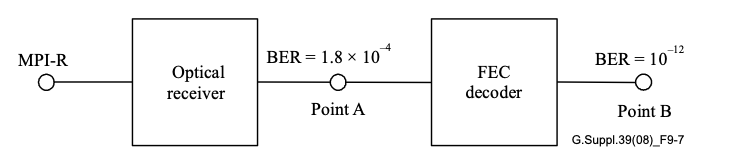
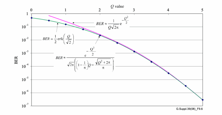
Forward Error Correction (FEC) has become an indispensable tool in modern optical communication, enhancing signal integrity and extending transmission distances. ITU-T recommendations, such as G.693, G.959.1, and G.698.1, define application codes for optical interfaces that incorporate FEC as specified in ITU-T G.709. In this blog, we discuss the significance of Bit Error Ratio (BER) in FEC-enabled applications and how it influences optical transmitter and receiver performance.

The Basics of FEC in Optical Communications

FEC is a method of error control for data transmission, where the sender adds redundant data to its messages. This allows the receiver to detect and correct errors without the need for retransmission. In the context of optical networks, FEC is particularly valuable because it can significantly lower the BER after decoding, thus ensuring the accuracy and reliability of data across vast distances.

BER Requirements in FEC-Enabled Applications

For certain optical transport unit rates (OTUk), the system BER is mandated to meet specific standards only after FEC correction has been applied. The optical parameters, in these scenarios, are designed to achieve a BER no worse than 10−12 at the FEC decoder’s output. This benchmark ensures that the data, once processed by the FEC decoder, maintains an extremely high level of accuracy, which is crucial for high-performance networks.

Practical Implications for Network Hardware

When it comes to testing and verifying the performance of optical hardware components intended for FEC-enabled applications, achieving a BER of 10−12 at the decoder’s output is often sufficient. Attempting to test components at 10−12 at the receiver output, prior to FEC decoding, can lead to unnecessarily stringent criteria that may not reflect the operational requirements of the application.

Adopting Appropriate BER Values for Testing

The selection of an appropriate BER for testing components depends on the specific application. Theoretical calculations suggest a BER of 1.8×10⁻⁴at the receiver output (Point A) to achieve a BER of 10−12 at the FEC decoder output (Point B). However, due to variations in error statistics, the average BER at Point A may need to be lower than the theoretical value to ensure the desired BER at Point B. In practice, a BER range of 10−5 to 10−6 is considered suitable for most applications.

Conservative Estimation for Receiver Sensitivity

By using a BER of 10−6 for component verification, the measurements of receiver sensitivity and optical path penalty at Point A will be conservative estimates of the values after FEC correction. This approach provides a practical and cost-effective method for ensuring component performance aligns with the rigorous demands of FEC-enabled systems.

Conclusion

FEC is a powerful mechanism that significantly improves the error tolerance of optical communication systems. By understanding and implementing appropriate BER testing methodologies, network operators can ensure their components are up to the task, ultimately leading to more reliable and efficient networks.

As the demands for data grow, the reliance on sophisticated FEC techniques will only increase, cementing BER as a fundamental metric in the design and evaluation of optical communication systems.

References

https://www.itu.int/rec/T-REC-G/e

Signal integrity is the cornerstone of effective fiber optic communication. In this sphere, two metrics stand paramount: Bit Error Ratio (BER) and Q factor. These indicators help engineers assess the performance of optical networks and ensure the fidelity of data transmission. But what do these terms mean, and how are they calculated?

What is BER?

BER represents the fraction of bits that have errors relative to the total number of bits sent in a transmission. It’s a direct indicator of the health of a communication link. The lower the BER, the more accurate and reliable the system.

ITU-T Standards Define BER Objectives

The ITU-T has set forth recommendations such as G.691, G.692, and G.959.1, which outline design objectives for optical systems, aiming for a BER no worse than 10−12 at the end of a system’s life. This is a rigorous standard that guarantees high reliability, crucial for SDH and OTN applications.

Measuring BER

Measuring BER, especially as low as 10−12, can be daunting due to the sheer volume of bits required to be tested. For instance, to confirm with 95% confidence that a system meets a BER of 10−12, one would need to test 3×1012 bits without encountering an error — a process that could take a prohibitively long time at lower transmission rates.

The Q Factor

The Q factor measures the signal-to-noise ratio at the decision point in a receiver’s circuitry. A higher Q factor translates to better signal quality. For a BER of 10−12, a Q factor of approximately 7.03 is needed. The relationship between Q factor and BER, when the threshold is optimally set, is given by the following equations:

The general formula relating Q to BER is:

bertoq

A common approximation for high Q values is:

ber_t_q_2

For a more accurate calculation across the entire range of Q, the formula is:

ber_t_q_3

Practical Example: Calculating BER from Q Factor

Let’s consider a practical example. If a system’s Q factor is measured at 7, what would be the approximate BER?

Using the approximation formula, we plug in the Q factor:

This would give us an approximate BER that’s indicative of a highly reliable system. For exact calculations, one would integrate the Gaussian error function as described in the more detailed equations.

Graphical Representation

ber_t_q_4

The graph typically illustrates these relationships, providing a visual representation of how the BER changes as the Q factor increases. This allows engineers to quickly assess the signal quality without long, drawn-out error measurements.

Concluding Thoughts

Understanding and applying BER and Q factor calculations is crucial for designing and maintaining robust optical communication systems. These concepts are not just academic; they directly impact the efficiency and reliability of the networks that underpin our modern digital world.

References

https://www.itu.int/rec/T-REC-G/e

Introduction

The telecommunications industry constantly strives to maximize the use of fiber optic capacity. Despite the broad spectral width of the conventional C-band, which offers over 40 THz, the limited use of optical channels at 10 or 40 Gbit/s results in substantial under utilization. The solution lies in Wavelength Division Multiplexing (WDM), a technique that can significantly increase the capacity of optical fibers.

Understanding Spectral Grids

WDM employs multiple optical carriers, each on a different wavelength, to transmit data simultaneously over a single fiber. This method vastly improves the efficiency of data transmission, as outlined in ITU-T Recommendations that define the spectral grids for WDM applications.

The Evolution of Channel Spacing

Historically, WDM systems have evolved to support an array of channel spacings. Initially, a 100 GHz grid was established, which was then subdivided by factors of two to create a variety of frequency grids, including:

  1. 12.5 GHz spacing
  2. 25 GHz spacing
  3. 50 GHz spacing
  4. 100 GHz spacing

All four frequency grids incorporate 193.1 THz and are not limited by frequency boundaries. Additionally, wider spacing grids can be achieved by using multiples of 100 GHz, such as 200 GHz, 300 GHz, and so on.

ITU-T Recommendations for DWDM

ITU-T Recommendations such as ITU-T G.692 and G.698 series outline applications utilizing these DWDM frequency grids. The recent addition of a flexible DWDM grid, as per Recommendation ITU-T G.694.1, allows for variable bit rates and modulation formats, optimizing the allocation of frequency slots to match specific bandwidth requirements.

Flexible DWDM Grid in Practice

#itu-t_grid

The flexible grid is particularly innovative, with nominal central frequencies at intervals of 6.25 GHz from 193.1 THz and slot widths based on 12.5 GHz increments. This flexibility ensures that the grid can adapt to a variety of transmission needs without overlap, as depicted in Figure above.

CWDM Wavelength Grid and Applications

Recommendation ITU-T G.694.2 defines the CWDM wavelength grid to support applications requiring simultaneous transmission of several wavelengths. The 20 nm channel spacing is a result of manufacturing tolerances, temperature variations, and the need for a guardband to use cost-effective filter technologies. These CWDM grids are further detailed in ITU-T G.695.

Conclusion

The strategic use of DWDM and CWDM grids, as defined by ITU-T Recommendations, is key to maximizing the capacity of fiber optic transmissions. With the introduction of flexible grids and ongoing advancements, we are witnessing a transformative period in fiber optic technology.

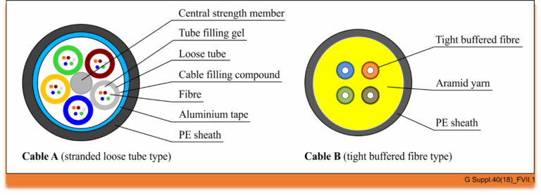
The world of optical communication is intricate, with different cable types designed for specific environments and applications. Today, we’re diving into the structure of two common types of optical fiber cables, as depicted in Figure below, and summarising the findings from an appendix that examined their performance.

cableA_B
#cable

Figure

Cable A: The Stranded Loose Tube Outdoor Cable

Cable A represents a quintessential outdoor cable, built to withstand the elements and the rigors of outdoor installation. The cross-section of this cable reveals a complex structure designed for durability and performance:

  • Central Strength Member: At its core, the cable has a central strength member that provides mechanical stability and ensures the cable can endure the tensions of installation.
  • Tube Filling Gel: Surrounding the central strength member are buffer tubes secured with a tube filling gel, which protects the fibers from moisture and physical stress.
  • Loose Tubes: These tubes hold the optical fibers loosely, allowing for expansion and contraction due to temperature changes without stressing the fibers themselves.
  • Fibers: Each tube houses six fibers, comprising various types specified by the ITU-T, including G.652.D, G.654.E, G.655.D, G.657.A1, G.657.A2, and G.657.B3. This array of fibers ensures compatibility with different transmission standards and conditions.
  • Aluminium Tape and PE Sheath: The aluminum tape provides a barrier against electromagnetic interference, while the polyethylene (PE) sheath offers physical protection and resistance to environmental factors.

The stranded loose tube design is particularly suited for long-distance outdoor applications, providing a robust solution for optical networks that span vast geographical areas.

Cable B: The Tight Buffered Indoor Cable

Switching our focus to indoor applications, Cable B is engineered for the unique demands of indoor environments:

  • Tight Buffered Fibers: Unlike Cable A, this indoor cable features four tight buffered fibers, which are more protected from physical damage and easier to handle during installation.
  • Aramid Yarn: Known for its strength and resistance to heat, aramid yarn is used to reinforce the cable, providing additional protection and tensile strength.
  • PE Sheath: Similar to Cable A, a PE sheath encloses the structure, offering a layer of defense against indoor environmental factors.

Cable B contains two ITU-T G.652.D fibers and two ITU-T G.657.B3 fibers, allowing for a blend of standard single-mode performance with the high bend-resistance characteristic of G.657.B3 fibers, making it ideal for complex indoor routing.

Conclusion

The intricate designs of optical fiber cables are tailored to their application environments. Cable A is optimized for outdoor use with a structure that guards against environmental challenges and mechanical stresses, while Cable B is designed for indoor use, where flexibility and ease of handling are paramount. By understanding the components and capabilities of these cables, network designers and installers can make informed decisions to ensure reliable and efficient optical communication systems.

Reference

https://www.itu.int/rec/T-REC-G.Sup40-201810-I/en

Items HD-FEC SD-FEC
Definition Decoding based on hard-bits(the output is quantized only to two levels) is called the “HD(hard-decision) decoding”, where each bit is considered definitely one or zero. Decoding based on soft-bits(the output is quantized to more than two levels) is called the “SD(soft-decision) decoding”, where not only one or zero decision but also confidence information for the decision are provided.
Application Generally for non-coherent detection optical systems, e.g.,  10 Gbit/s, 40 Gbit/s, also for some coherent detection optical systems with higher OSNR coherent detection optical systems, e.g.,  100 Gbit/s,400 Gbit/s.
Electronics Requirement ADC(Analogue-to-Digital Converter) is not necessary in the receiver. ADC is required in the receiver to provide soft information, e.g.,  coherent detection optical systems.
specification general FEC per [ITU-T G.975];super FEC per [ITU-T G.975.1]. vendor specific
typical scheme Concatenated RS/BCH LDPC(Low density parity check),TPC(Turbo product code)
complexity medium high
redundancy ratio generally 7% around 20%
NCG about 5.6 dB for general FEC;>8.0 dB for super FEC. >10.0 dB
 Example(If you asked your friend about traffic jam status on roads and he replies) maybe fully jammed or free  50-50  but I found othe way free or less traffic