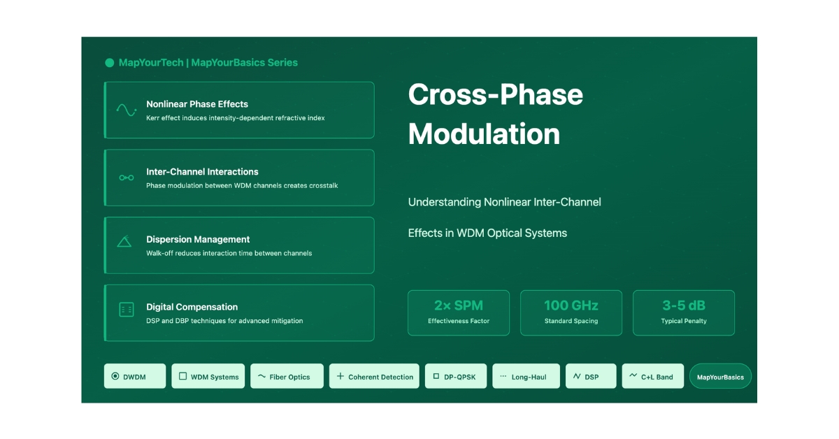
Cross-Phase Modulation

Understanding Nonlinear Inter-Channel Interactions in WDM Systems

MapYourTech | MapYourBasics Series

Fundamentals & Core Concepts

What is Cross-Phase Modulation?

Cross-Phase Modulation (XPM) is a nonlinear effect in optical fiber communications that results from the intensity-dependent refractive index of the fiber. In Wavelength Division Multiplexing (WDM) systems, when two or more optical signals travel simultaneously through the same fiber, the optical power of one signal can influence the phase of other signals, leading to XPM-induced distortions.

                Key Definition: XPM describes the interaction between adjacent channels (inter-channel cross-phase modulation) where the refractive index of the fiber is affected by the combined optical power of all copropagating channels. This variation in refractive index leads to phase shifts in all channels, causing timing jitter, phase noise, and spectral broadening.
            

Why Does XPM Occur?

XPM originates from the Kerr nonlinearity of optical fibers, where the refractive index varies in proportion to the intensity of propagating signals. The physical mechanism can be understood through the following principles:

Kerr Effect Mechanism:

The refractive index of an optical fiber changes in response to the optical power traveling through it:

n = n₀ + n₂ · I

where n₀ is the linear refractive index, n₂ is the nonlinear index coefficient, and I is the intensity of the optical signal.

XPM is twice as effective as Self-Phase Modulation (SPM) because the intensity of neighboring channels contributes to the total phase shift experienced by the signal. This inter-channel interaction distorts the signal, causing timing jitter, phase noise, and spectral broadening.

When Does XPM Matter?

XPM becomes particularly problematic in Dense Wavelength Division Multiplexing (DWDM) systems under the following conditions:

Narrow Channel Spacing: Systems with 50 GHz or 100 GHz channel spacing in DWDM systems experience significant XPM effects
High Channel Power: Increased optical power strengthens the nonlinear interaction between channels
Low Fiber Dispersion: Reduced dispersion allows longer interaction times between channels
Long-Haul Systems: Multi-span systems with EDFA amplifiers accumulate XPM-induced noise and phase distortions
High Bit Rates: Systems above 10 Gbit/s with broader signal spectra experience increased intra-channel XPM (IXPM)

Why is XPM Important?

Understanding and managing XPM is important for modern optical networks because it:

Impact Area	Effect	Consequence
Signal Quality	Phase modulation between channels	Degraded signal integrity and increased BER
Timing	Pattern-dependent phase shifts	Timing jitter that varies with bit patterns
OSNR	Inter-channel interference	Reduced optical signal-to-noise ratio
System Reach	Cumulative distortion over spans	Limited transmission distance
Capacity	Channel spacing constraints	Reduced spectral efficiency

                Real-World Analogy: Think of XPM like multiple boats traveling in a narrow canal. As one boat creates waves (phase distortions), these waves affect the stability and course of nearby boats. The closer the boats (channels) are together and the faster they move (higher power), the more they interfere with each other's smooth passage.
            

Mathematical Framework

Core XPM Phase Shift Equation

Nonlinear Phase Shift for Channel i

φ_i,NL = γ · L_eff · [P_i + 2 · Σ(P_j)]

Where:

φ_i,NL: Total nonlinear phase shift for channel i (radians)
γ: Nonlinear coefficient of the fiber (W^-1km^-1), related to fiber effective area and nonlinear refractive index
L_eff: Effective length of the fiber (km)
P_i: Power of the i-th channel (W)
P_j: Power of the j-th interfering channel (W)

XPM-Induced Frequency Chirp

Frequency Shift Due to XPM

δω_XPM = -2γ · L_eff · (dI(t)/dt)

Interpretation: The XPM-induced chirp is proportional to the time derivative of the signal's intensity. This shows that the frequency shift depends on how quickly the optical power changes in the copropagating channels.

Effective Length Calculation

Fiber Effective Length

L_eff = (1 - e^-αL) / α

Parameters:

α: Fiber loss coefficient (km^-1), typically 0.2 dB/km at 1550 nm
L: Physical fiber length (km)

For long fibers where αL &Gt; 1, L_eff ≈ 1/α

Simplified XPM Phase Shift (Two Channels)

Phase Shift with Two Copropagating Channels

φ_XPM = 2γ · L_eff · P_other

This equation shows that XPM effects are twice as strong as SPM effects (factor of 2), making inter-channel interactions particularly significant in WDM systems.

Practical Example — XPM Phase Shift in a DWDM Link

System Parameters:

Fiber length (L) = 100 km
Fiber attenuation (α) = 0.2 dB/km = 0.046 km^-1
Nonlinear coefficient (γ) = 1.3 W^-1km^-1
Channel power (P_i) = 1 mW = 0.001 W
Number of interfering channels = 50

Step 1: Calculate Effective Length

L_eff = (1 - e^{-(0.046 × 100)}) / 0.046 = (1 - 0.01) / 0.046 ≈ 21.5 km

Step 2: Calculate Total XPM Phase Shift

φ_XPM = 2 × 1.3 × 21.5 × (50 × 0.001) = 2.795 radians ≈ 160°

Result: The XPM-induced phase shift of approximately 160° is significant and will cause noticeable signal degradation, requiring mitigation such as dispersion management or power reduction.

XPM Power Penalty Estimation

Maximum Phase Shift Condition

φ_max = (γ/α) · (2N - 1) · P_ch

Design Rule: To limit XPM effects, keep φ_max < 1 radian

P_ch < α / [γ · (2N - 1)]

For N > 50 channels with typical α and γ values, channel power should be below 1 mW to minimize XPM-induced penalties.

Types & Components

Classification of XPM Effects

1. Inter-Channel Cross-Phase Modulation

The classical XPM effect describing interactions between different wavelength channels in WDM systems.

Characteristics:

Occurs between adjacent or nearby wavelength channels
Strength depends on channel spacing (50 GHz, 100 GHz)
Most significant for closely spaced DWDM channels
Affected by dispersion-induced walk-off between channels
Dominant in systems with low-to-moderate dispersion

2. Intra-Channel Cross-Phase Modulation (IXPM)

XPM interactions within a single channel, becoming dominant at bit rates above 10 Gbit/s with broader signal spectra.

Key Features:

Interaction between pulses within the same channel
Introduces timing jitter in pseudo-linear systems
Becomes a dominating factor at higher bit rates (>10 Gbit/s)
Causes both amplitude and timing fluctuations
Interacts with ASE noise to produce phase jitter

Component Breakdown: XPM in System Context

Component	Role in XPM	Impact
Optical Fiber	Nonlinear medium where XPM occurs	Fiber type (SMF, NZDSF) determines XPM severity through γ and dispersion
WDM Channels	Interacting optical signals	Channel power and spacing determine XPM strength
EDFA Amplifiers	Power restoration points	Create power variations that enhance XPM asymmetry
Dispersion	Walk-off mechanism	Controls interaction time between channels
Modulation Format	Signal characteristics	ASK more sensitive to XPM than PSK formats

XPM vs. SPM vs. FWM Comparison

Characteristic	XPM	SPM	FWM
Interaction Type	Inter-channel	Self-channel	Multi-channel mixing
Effectiveness Factor	2× relative to SPM	Baseline (1×)	Phase-matched
Primary Effect	Phase modulation	Spectral broadening	New frequencies
Dispersion Sensitivity	Moderate (walk-off)	Low	High (phase matching)
Channel Spacing Impact	Strong	None	Very strong
Power Threshold	~+7 dBm	~+8 dBm	~+3 dBm
Mitigation Strategy	Dispersion management, channel spacing	Power reduction, dispersion compensation	Increase dispersion, wider spacing

XPM in Different System Scenarios

Short-Haul Systems (< 200 km)

XPM Impact: Limited due to relatively short fiber lengths and lower accumulated nonlinear effects.

Typical Power Levels: Can operate at higher channel powers (> 0 dBm) without significant XPM penalties.

Mitigation: Often minimal mitigation required; basic power management sufficient.

Long-Haul Systems (> 1000 km)

XPM Impact: A significant issue requiring careful management. Cumulative XPM across multiple spans with EDFA amplifiers severely degrades performance.

Typical Power Levels: Requires reduced channel power (< 0 dBm) and careful dispersion management.

Mitigation: Comprehensive approach including dispersion management, power equalization, and possibly digital compensation.

Effects & Impacts

System-Level Effects of XPM

1. Timing Jitter

XPM-induced phase modulation causes fluctuations in the timing of signal pulses. The mechanism works as follows:

Timing Jitter Mechanism:

Pattern-dependent phase shifts → Frequency chirping → Changes in group velocity → Pulse position shifts

The temporal shift depends on the bit pattern surrounding each pulse, varying from bit to bit based on transmitted data. This creates timing uncertainty at the receiver, degrading system performance.

Timing jitter increases with the number of WDM channels
Jitter magnitude proportional to overall channel power
Most severe when pulse widths are comparable to bit slot spacing
Can be reduced by stretching pulses over multiple bit slots (pseudo-linear systems)

2. Spectral Broadening

XPM gradually broadens the signal spectrum as changes in optical intensity result in phase variations. The spectral broadening mechanism involves:

Broadening Process:

Intensity variations in copropagating channels create time-dependent phase shifts
Phase variations translate to frequency chirping across the pulse
Spectral components spread beyond original bandwidth
Chromatic dispersion then causes temporal broadening of the broadened spectrum

The amount of spectral broadening relates to transmission signal rate, channel separation, and fiber chromatic dispersion. Dispersion-induced differential group velocities cause interacting pulses to separate during propagation, limiting the interaction length.

3. Power Fluctuations

XPM converts pattern-dependent phase shifts into power fluctuations through fiber dispersion. Observed effects include:

CW probe power can fluctuate by 6% or more after a few hundred kilometers
Fluctuation extent depends on channel power and dispersion
Asymmetric pulse collisions in amplified systems create net frequency shifts
Results in amplitude jitter varying with bit patterns

Performance Impact Quantification

OSNR Degradation

XPM affects the optical signal-to-noise ratio through inter-channel interference, particularly in long-haul systems with multiple fiber spans. The phase modulation from XPM degrades OSNR and increases bit error rate (BER).

System Parameter	Impact on XPM	OSNR Effect
Channel Count (N)	Linear increase in XPM	~0.5-1 dB penalty per 10 channels
Channel Spacing	Inverse relationship	2-3 dB worse at 50 GHz vs 100 GHz
Channel Power	Linear with power	~1 dB penalty per 1 dBm increase
Transmission Distance	Cumulative effect	3-5 dB total over transoceanic

Power Penalty Analysis

XPM-Induced Power Penalty

Power penalty arises from signal distortion that reduces SNR and leads to bit errors. As WDM channel count increases, XPM power penalty becomes more significant.

Typical Penalty Values:

10-channel system, 100 GHz spacing: 0.5-1 dB
40-channel system, 100 GHz spacing: 2-3 dB
40-channel system, 50 GHz spacing: 4-6 dB
Can exceed 5 dB for closely spaced channels in long systems

Threshold Levels and Tolerance

Parameter	Threshold Value	Consequence if Exceeded
Nonlinear Phase Shift	< 1 radian	Strong nonlinear distortion region
Channel Power (N > 50)	< 1 mW (0 dBm)	Excessive XPM-induced penalties
Channel Spacing (DWDM)	> 50 GHz	Increased inter-channel interaction
Fiber Effective Area	> 80 μm²	Higher nonlinear coefficient γ
System Reach (without mitigation)	< 1000 km	Cumulative XPM limits distance

Mitigation Strategies Overview

1. Dispersion Management: Managing fiber dispersion reduces interaction time between channels by causing pulse walk-off. This is the most effective technique for controlling XPM in WDM systems.

2. Channel Spacing Optimization: Increasing spacing to 100 GHz or greater reduces XPM between channels, at the cost of spectral efficiency.

3. Power Reduction: Lowering channel power directly reduces XPM strength, but must be balanced against OSNR requirements and transmission reach.

4. Advanced Modulation Formats: PSK formats (QPSK, DPSK) with constant amplitude are less affected by XPM than ASK formats, though they remain sensitive to phase noise.

Techniques & Solutions

1. Dispersion Management Techniques

Dispersion management is the most effective approach for mitigating XPM by reducing the interaction time between channels through controlled pulse walk-off.

Dispersion Compensation Methods

Method	Implementation	Advantages	Disadvantages
DCF (Dispersion Compensating Fiber)	Negative dispersion fiber modules at intervals	Proven technology, effective for XPM control	Adds loss, requires amplification
Fiber Bragg Gratings	Wavelength-selective reflectors	Compact, low loss, can introduce time delays	Wavelength-specific, limited bandwidth
DSP-Based Compensation	Digital signal processing at receiver	Flexible, no optical components needed	Computational complexity, power consumption
Dispersion Maps	Alternating positive/negative dispersion sections	Optimizes both SPM and XPM performance	Complex design, system-specific

Dispersion Map Design Principles

Objective: Create an optimal balance between limiting nonlinear effects and controlling pulse broadening.

Local dispersion should be relatively large to induce walk-off between channels
End-to-end accumulated dispersion must stay within acceptable limits
Typical approach: alternate between anomalous and normal dispersion sections
Compensation interval: every 50-100 km in long-haul systems
Must avoid zero-dispersion wavelengths to prevent FWM

2. Channel Spacing Optimization

Increasing the spectral separation between channels reduces XPM by decreasing the phase modulation overlap.

Channel Spacing	XPM Impact	Spectral Efficiency	Best Application
25 GHz	Very High	Maximum	Short reach, metro systems
50 GHz	High	High	Regional networks with careful management
100 GHz	Moderate	Medium	Long-haul DWDM (most common)
200 GHz	Low	Lower	Ultra-long-haul, transoceanic
CWDM (20 nm)	Negligible	Very Low	Metro access, limited channel count

3. Power Management Techniques

Power Reduction Strategy

Principle: Since XPM is directly proportional to channel power, reducing optical power decreases nonlinear interactions.

Implementation Approaches:

Per-Channel Power Control: Optimize power for each wavelength individually
Launch Power Optimization: Balance between OSNR requirements and XPM limits
Raman Amplification: Distributed gain reduces peak powers along the fiber
Dynamic Power Adjustment: Adapt power based on channel loading and network conditions

Design Rule: For N > 50 channels, maintain P_ch < α/[γ(2N-1)] ≈ 1 mW to keep φ_max < 1 radian

Power Equalization

Ensuring balanced power levels across all channels prevents high-power channels from disproportionately affecting weaker channels through XPM.

Techniques:

Variable optical attenuators (VOAs) at transmitters
Gain equalizing filters in amplifier chains
Per-channel power monitoring and feedback control
Wavelength-dependent loss compensation

4. Advanced Modulation Formats

The choice of modulation format affects XPM sensitivity:

Modulation Format	XPM Sensitivity	Key Characteristics	Typical Use Case
OOK/ASK	High	Large intensity variations make it vulnerable to XPM	Legacy 10G systems
DPSK	Moderate	Constant amplitude reduces XPM impact	40G long-haul
QPSK	Low-Moderate	Constant envelope, primarily sensitive to phase noise	100G coherent systems
16QAM	Moderate-High	Amplitude variations increase XPM sensitivity	200G/400G metro and regional
64QAM	High	Complex constellation very sensitive to distortions	Short reach high capacity

5. Polarization Techniques

Polarization Multiplexing

Since XPM is polarization-dependent, using orthogonal polarization states can reduce inter-channel interactions.

Strategy: Ensure neighboring channels have orthogonal polarization states to minimize XPM-induced phase shifts.

Benefits:

Reduces effective XPM coefficient by a factor related to polarization overlap
Doubles spectral efficiency when used with PDM formats
Particularly effective in coherent detection systems

Challenges:

Polarization mode dispersion (PMD) can scramble polarization states
Requires careful control along the entire link
Cross-polarization modulation (XPolM) can still occur

6. Digital Signal Processing (DSP) Solutions

Digital Back Propagation (DBP)

DBP is a powerful technique that computationally reverses fiber transmission effects, including XPM.

How DBP Works:

At the receiver, implement the inverse nonlinear Schrödinger equation
Numerically propagate the signal backward through a virtual fiber
Compensate for both dispersion and nonlinear effects (SPM, XPM)
Recover the original transmitted signal

Performance: Can provide 4-6 dB Q-factor improvement when compensating XPM in WDM systems. Particularly effective in dispersion-unmanaged transmission.

Limitation: High computational complexity. XPM compensation requires processing all WDM channels simultaneously, increasing complexity ~300× compared to dispersion-only compensation.

Pilot Tone Equalization

Technique: Insert a pilot tone next to the WDM channel and propagate together. At the coherent receiver, extract phase information from the tone containing XPM effects from other channels, then subtract this XPM contribution to remove phase distortion.

Effectiveness: Proven efficient when combined with intrachannel SPM compensation, particularly helpful for high-order modulations.

Best Practices and Recommendations

Recommended Approach for Different Scenarios

Metro Networks (< 200 km):

Basic power management usually sufficient
50 GHz channel spacing acceptable with moderate power
Simple dispersion compensation if needed

Regional Networks (200-1000 km):

Implement dispersion management every 100-200 km
Use 100 GHz channel spacing
Optimize launch power (typically -2 to 0 dBm per channel)
Consider QPSK or DPSK modulation formats

Long-Haul/Transoceanic (> 1000 km):

Comprehensive dispersion map design essential
100-200 GHz channel spacing recommended
Reduced launch power (< -2 dBm per channel)
Consider Raman amplification for distributed gain
Use coherent detection with DSP compensation
Implement digital back propagation if feasible

Design Guidelines & Method

Step-by-Step Design Process

                Phase 1: System Requirements Analysis
                Define System Parameters: Transmission distance, number of channels, data rates, modulation formats
Establish Performance Targets: Required BER (typically 10-12), OSNR margin, maximum acceptable penalty
Identify Constraints: Fiber type availability, amplifier spacing, budget limitations
Determine Critical Thresholds: Maximum nonlinear phase shift (< 1 radian), power budgets

            

                Phase 2: XPM Impact Assessment
                Calculate Nonlinear Coefficient: γ = 2πn2/(λAeff), typical range 1-2 W-1km-1
Estimate Effective Length: Leff = (1 - e-αL)/α for each span
Compute Phase Shift: φXPM = 2γLeff · Σ(Pj) for worst-case channel
Assess Walk-off Length: to determine interaction length between channels
Estimate Power Penalty: Based on channel count, spacing, and system length

            

                Phase 3: Mitigation Strategy Selection
                Channel Spacing Decision: Select 50, 100, or 200 GHz based on XPM severity and capacity requirements
Power Optimization: Determine optimal launch power balancing OSNR vs XPM
Dispersion Management: Design a dispersion map with compensation intervals
Modulation Format: Choose a format appropriate for distance and XPM sensitivity
Advanced Techniques: Evaluate the need for DSP compensation, Raman amplification

            

                Phase 4: Implementation and Verification
                Deploy System: Install fibers, amplifiers, DCF modules as per design
Commissioning Tests: Measure OSNR, BER, Q-factor for all channels
Optimization: Fine-tune power levels, verify dispersion compensation
Performance Monitoring: Establish baseline and ongoing monitoring protocols

            

Decision Framework

If XPM Penalty is...	And Distance is...	Then Recommended Action is...
< 0.5 dB	Any	No special mitigation needed, maintain current configuration
0.5-2 dB	< 500 km	Basic power optimization sufficient
0.5-2 dB	> 500 km	Implement dispersion compensation at regular intervals
2-5 dB	< 1000 km	Increase channel spacing to 100 GHz + dispersion management
2-5 dB	> 1000 km	Comprehensive approach: wider spacing, power reduction, advanced DSP
> 5 dB	Any	Major system redesign: consider 200 GHz spacing, Raman amplification, DBP

Practical Example — 40-Channel DWDM System Design

Requirements:

Distance: 800 km
Data rate: 100 Gbps per channel
Number of channels: 40
Target BER: < 10^-12

Step 1: Initial Calculations

Fiber: SMF with γ = 1.3 W^-1km^-1, α = 0.2 dB/km, D = 17 ps/nm/km
Span length: 80 km, Number of spans: 10, L_eff per span: 21.5 km

Step 2: XPM Assessment

Trial with 50 GHz spacing and 2 mW per channel:

φ_XPM = 2 × 1.3 × 21.5 × (39 × 0.002) = 4.35 radians per span → ~43 radians over 10 spans → unacceptable.

Step 3: Design Optimization

Use 100 GHz spacing with 0.5 mW (-3 dBm) per channel:

φ_XPM = 2 × 1.3 × 21.5 × (39 × 0.0005) = 1.09 radians per span. With dispersion management reducing effective interaction to ~0.6 radians per span: ~6 radians over 10 spans → acceptable with a proper dispersion map.

Step 4: Dispersion Management

Install DCF modules every 160 km (2 spans)
Each DCF compensates -1360 ps/nm (80 km × 17 ps/nm/km)
Local dispersion in transmission fiber: 17 ps/nm/km (induces walk-off)
Local dispersion in DCF: -100 ps/nm/km

Step 5: Modulation Format Selection

Choose DP-QPSK for 100G: constant envelope reduces XPM sensitivity; coherent detection allows DSP compensation; good balance of reach and spectral efficiency.

Expected Performance:

XPM penalty: ~2 dB
Total OSNR requirement: 15 dB (12 dB for QPSK + 3 dB margin)
Achievable with EDFA amplification and proper power management

Common Pitfalls to Avoid

Issue	Why It's a Problem	How to Avoid
Ignoring XPM in initial design	Leads to unexpected penalties and BER degradation after deployment	Always include XPM assessment in link budget calculations
Using overly optimistic power levels	Causes severe nonlinear penalties that limit system reach	Follow power guidelines: < 0 dBm for dense WDM systems
Inadequate dispersion compensation	Allows prolonged channel interactions, maximizing XPM effects	Design a proper dispersion map with regular compensation
Neglecting channel count scaling	XPM scales linearly with the number of interfering channels	Reassess design when adding channels to existing systems
Inconsistent power across channels	High-power channels disproportionately affect weak channels	Implement power equalization across all wavelengths
Wrong modulation format choice	High-order QAM very sensitive to XPM amplitude fluctuations	Match format to distance: QPSK for long-haul, QAM for short reach

Interactive Simulators

Four calculators let you build intuition for how XPM scales with power, channel count, distance, and spacing. Use the tabs to switch between the phase-shift calculator, the channel-spacing comparison, the multi-span impact analysis, and the system optimizer. All inputs carry units and sensible defaults; results show a pass/marginal/fail band.

Takeaway: These models use the simplified phase-shift relation and an illustrative penalty mapping for teaching. They are good for sizing the order of magnitude of XPM; production link engineering uses a full Gaussian-Noise or split-step model with measured fiber parameters.

Practical Applications & Case Studies

Real-World Deployment Scenarios

Scenario 1: Metro/Regional DWDM Network

Application: High-capacity metro network connecting data centers within a metropolitan area

System Configuration:

Distance: 50-200 km
Channel count: 80-96 channels (C-band)
Channel spacing: 50 GHz
Data rate: 100G per channel
Modulation: DP-QPSK

XPM Considerations:

Relatively short distances reduce cumulative XPM effects
High channel count requires careful power management
Dense 50 GHz spacing increases XPM interactions
Typical XPM penalty: 1-2 dB

Mitigation Strategy: Per-channel power optimization at 0-2 dBm, basic dispersion pre-compensation, power equalization across wavelengths.

Scenario 2: Long-Haul Terrestrial Network

Application: Cross-country backbone network connecting major cities

System Configuration:

Distance: 1500-2500 km
Channel count: 40-80 channels
Channel spacing: 100 GHz
Data rate: 100-200G per channel
Span length: 80-100 km with EDFA

XPM Considerations:

Long distances cause significant cumulative XPM
Multiple amplified spans increase power variations
Typical XPM penalty: 3-5 dB without proper management
Interaction with chromatic dispersion is important

Mitigation Strategy: Comprehensive dispersion map with DCF every 160-200 km, reduced launch power (-2 to 0 dBm), hybrid Raman/EDFA amplification, coherent detection with DSP compensation.

Scenario 3: Transoceanic Submarine System

Application: Undersea cable system connecting continents

System Configuration:

Distance: 6000-10000 km
Channel count: 40-100 channels (C+L band)
Channel spacing: 100-200 GHz
Data rate: 100-200G per channel
Modulation: DP-QPSK or DP-16QAM

XPM Considerations:

Extreme distances require stringent XPM control
Hundreds of spans accumulate nonlinear effects
Must optimize for maximum capacity and reach
XPM can limit achievable capacity

Mitigation Strategy: Carefully designed dispersion map, very low launch power (-3 to -1 dBm), 100-200 GHz channel spacing, advanced DSP including digital back propagation, possibly lower-order modulation (QPSK) for maximum reach.

Case Study 1: Upgrading Metro Network Capacity

Challenge

A telecommunications operator needed to upgrade a 200 km metro DWDM network from 40 channels at 10G each (400G total) to 80 channels at 100G each to meet growing bandwidth demands. The existing system used 100 GHz channel spacing.

Problem Encountered

Initial deployment with 50 GHz spacing and 2 mW per channel resulted in:

BER exceeding 10^-9 on most channels (target was 10^-12)
OSNR degradation of 4-5 dB attributed to XPM
Significant timing jitter observed on the spectrum analyzer
Worst affected channels were in the center of the C-band

Analysis

Calculated XPM phase shift: φ_XPM ≈ 4.2 radians (unacceptable)
50 GHz spacing insufficient for 80-channel system at this power
Close spacing with high power created severe inter-channel crosstalk
Existing SMF fiber with γ = 1.3 W^-1km^-1 contributed to high nonlinearity

Solution Implemented

Return to 100 GHz Spacing: Reduced to 40 channels at 100G (4T total capacity)
Power Optimization: Reduced launch power from 2 mW to 0.8 mW (-1 dBm) per channel
Power Equalization: Implemented VOAs for ±0.5 dB power uniformity across all channels
Modulation Upgrade: Used DP-QPSK instead of intensity modulation for better XPM tolerance
Basic Dispersion Management: Added pre-compensation modules at transmitters

Results

BER improved to < 10^-12 on all channels
XPM penalty reduced to < 1.5 dB
OSNR margin improved by 3 dB
Achieved 4T capacity (10× original capacity)
System stable and ready for future C+L band expansion

Case Study 2: Long-Haul System Optimization

Challenge

An operator was deploying a new 1600 km long-haul system with 40 channels at 100G each, targeting transmission without regeneration while maintaining BER < 10^-12.

Initial Design Issues

Used 100 GHz spacing with 1 mW (0 dBm) per channel
80 km span length with EDFA amplifiers
Minimal dispersion compensation (only at endpoints)
Result: BER floors at 10^-6 on several channels; cumulative XPM over 20 spans caused severe degradation

Engineering Solution

Dispersion Compensation: Installed DCF modules every 160 km (2 spans)
Map Structure: Each section: 2× 80 km SMF (D = +17 ps/nm/km) + DCF (D = -100 ps/nm/km)
Local Dispersion: Maintained high local dispersion to induce walk-off
Power Reduction: Lowered launch power to 0.5 mW (-3 dBm) per channel
Hybrid Amplification: Added Raman pumps to reduce required EDFA gain
DSP Implementation: Enabled chromatic dispersion and XPM compensation at coherent receivers

Performance Achieved

BER < 10^-12 on all 40 channels
XPM penalty reduced from ~6 dB to < 2 dB
3 dB OSNR margin; regeneration-free transmission over 1600 km
Walk-off from the dispersion map reduced XPM interaction time by ~60%

Case Study 3: C+L Band Expansion with XPM Management

Challenge

A submarine cable operator needed to double the capacity of an existing 5000 km transoceanic system by expanding from C-band only (40 channels) to C+L band (80 channels total).

Unique Complications

Cannot modify existing submarine infrastructure (amplifiers, fiber)
Adding L-band channels increases total optical power in fiber
XPM between C and L bands must be managed
Stimulated Raman Scattering (SRS) transfers power from C to L band
Both XPM and SRS create power tilt across bands

Solution

Power Rebalancing: Reduced C-band channel power by 1 dB, increased L-band by 0.5 dB to compensate for SRS
Pre-Distortion: Applied pre-emphasis at the transmitter for expected power tilt
Wider L-Band Spacing: 200 GHz for L-band channels vs 100 GHz for C-band
Modulation: Maintained DP-QPSK for reliability at ultra-long distances
DSP: Implemented joint C+L band nonlinear compensation

Results and Impact

Doubled system capacity to 8 Tbps
Inter-band XPM penalty limited to < 2 dB through careful power management
All 80 channels achieving target BER < 10^-15 (with FEC)
Power tilt across C+L bands maintained within ±1 dB

Troubleshooting Guide

Symptom	Likely XPM-Related Cause	Diagnostic Steps	Recommended Fix
BER floor above target	Excessive XPM causing timing/amplitude jitter	Measure OSNR on all channels; check pattern-dependent errors; calculate φ_XPM	Reduce launch power or increase channel spacing
Center channels worse than edge	Maximum XPM on center channels from all neighbors	Compare BER across wavelengths; verify power equalization; check for FWM products	Implement per-channel power optimization
Performance degrades with distance	Cumulative XPM over multiple spans	Test at intermediate points; measure dispersion; verify amplifier gains	Add dispersion compensation or reduce power
Timing jitter observed	XPM-induced frequency shifts via GVD	Use sampling scope; check pulse shapes; measure jitter statistics	Improve dispersion management
Power fluctuations on spectrum	XPM converting phase to amplitude via dispersion	Use OSA to monitor; check modulation format; verify fiber dispersion	Add pre-compensation or change modulation
Degradation after adding channels	Increased total XPM from more interferers	Compare before/after performance; recalculate φ_XPM; measure crosstalk	Reoptimize power for new channel count

Quick Reference: XPM Mitigation by System Type

System Type	Primary Strategy	Secondary Strategies	Typical XPM Penalty
Metro (< 200 km)	Power optimization	Basic dispersion pre-comp, 50-100 GHz spacing	0.5-2 dB
Regional (200-1000 km)	Dispersion management	100 GHz spacing, power reduction, QPSK modulation	1-3 dB
Long-Haul (1000-3000 km)	Comprehensive disp. map	Reduced power, Raman amp, coherent detection + DSP	2-4 dB
Ultra-Long (> 3000 km)	Optimized disp. map + DBP	100-200 GHz spacing, very low power, advanced FEC	3-5 dB
High-Density (80+ channels)	Channel spacing increase	Per-channel power control, power equalization	2-5 dB

Main Points

XPM is a nonlinear effect in WDM systems caused by the intensity-dependent refractive index, producing inter-channel phase modulation.
XPM is twice as effective as SPM, making it particularly significant in dense DWDM systems with many copropagating channels.
Primary effects are timing jitter, spectral broadening, and power fluctuations, leading to OSNR degradation and increased BER.
XPM penalty scales linearly with channel count and power, and inversely with channel spacing.
Dispersion management is the most effective mitigation, using walk-off to reduce interaction time between channels.
For systems with φ_XPM > 1 radian, significant performance degradation occurs and mitigation is needed.
Channel spacing selection matters: 50 GHz needs stringent management, 100 GHz is standard for long-haul, 200 GHz for ultra-long distances.
Power optimization must balance XPM reduction against OSNR, typically keeping per-channel power below 0 dBm for N > 50 channels.
Constant-amplitude formats (QPSK, DPSK) tolerate XPM better than intensity-modulated formats (OOK, QAM).
DSP techniques, including digital back propagation, can give 4-6 dB improvement but at high computational cost.

References

ITU-T G.652 — Characteristics of a Single-Mode Optical Fibre and Cable, ITU-T Study Group 15.
ITU-T G.663 — Application-Related Aspects of Optical Amplifier Devices and Subsystems, ITU-T Study Group 15.
G. P. Agrawal — Nonlinear Fiber Optics, Academic Press.
Sanjay Yadav, "Optical Network Communications: An Engineer's Perspective" — Bridge the Gap Between Theory and Practice in Optical Networking.

Developed by MapYourTech Team

For educational purposes in Optical Networking Communications Technologies

Note: This guide is based on industry standards, best practices, and real-world implementation experiences. Specific implementations may vary based on equipment vendors, network topology, and regulatory requirements. Always consult with qualified network engineers and follow vendor documentation for actual deployments.

Feedback Welcome: If you have any suggestions, corrections, or improvements to propose, please write to us at [email protected]