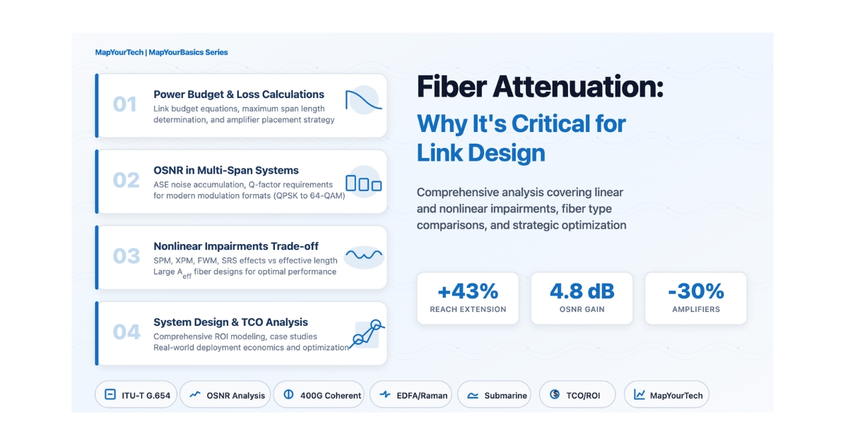

Fiber Attenuation: Why It's Critical for Optical Link Design
Comprehensive Technical Analysis of Linear and Nonlinear Impairments
1. Executive Summary
Fiber attenuation is the single most critical parameter in optical network design, directly determining maximum transmission distance, amplifier spacing, system OSNR, and overall network economics. A reduction in attenuation from 0.20 to 0.14 dB/km enables 43% longer unregenerated spans, improves OSNR by 4.8 dB in multi-span systems, and can reduce amplifier counts by up to 29% in long-haul deployments—but simultaneously increases nonlinear effective length by 33%, creating a fundamental trade-off that shapes every aspect of modern optical systems.
Key Discoveries:
- Linear Performance Boost: Ultra-low-loss (ULL) fiber achieving 0.14 dB/km extends maximum unregenerated reach from 115 km to 164 km with typical 100G transceivers
- OSNR Enhancement: In a 4,000 km system with 80 km spans, reducing loss from 0.20 to 0.14 dB/km improves OSNR by 4.8 dB—enabling 64-QAM modulation where only 16-QAM was previously viable
- Amplifier Economics: A 9,000 km transoceanic cable using 70 km spans (enabled by ULL fiber) versus 50 km spans saves 51 submarine repeaters at hundreds of thousands of dollars each
- Nonlinear Trade-off: Lower attenuation increases effective length (Leff) from 22 km to 29 km, requiring careful power management to avoid self-phase modulation and four-wave mixing penalties
2. Introduction and Fundamentals
2.1 What is Fiber Attenuation?
Fiber attenuation measures the exponential decay of optical signal power as light propagates through silica glass, universally expressed in decibels per kilometer (dB/km). This seemingly simple metric fundamentally drives nearly every major design decision in optical networks—from maximum unregenerated transmission distance to the number and spacing of expensive optical amplifiers in long-haul systems.
The mathematical relationship governing signal power decay follows an exponential function:
P(L) = P₀ × 10(-αL/10)
or equivalently in logarithmic form:
Loss (dB) = 10 × log₁₀(P₀/Pout) = α × L
Where:
• P(L) = Output power after distance L
• P₀ = Initial launched power
• α = Attenuation coefficient (dB/km)
• L = Fiber length (km)
For example, a signal at 0 dBm (1 mW) traversing 100 km of fiber with 0.20 dB/km attenuation emerges at:
Pout = 0 dBm - 20 dB = -20 dBm (10 μW)
Linear power ratio: Pout/P₀ = 10(-20/10) = 0.01 (1% of original power)
2.2 Physical Mechanisms of Attenuation
2.2.1 Rayleigh Scattering: The Dominant Loss Mechanism
Rayleigh scattering accounts for approximately 96% of attenuation in modern optical fibers. This fundamental physical phenomenon arises from microscopic density fluctuations frozen into the glass structure during the manufacturing process. These sub-wavelength inhomogeneities (on the order of 0.1-1 nm) scatter light in all directions, with intensity following an inverse fourth-power wavelength dependence:
αRayleigh ∝ λ-4
More precisely:
αRayleigh(λ) = (8π³/3λ⁴) × n⁸ × p² × kB × Tf × βT
Where:
• λ = wavelength of light
• n = refractive index (~1.46 for silica)
• p = photoelastic coefficient
• kB = Boltzmann constant
• Tf = fictive temperature (~1,500 K)
• βT = isothermal compressibility
This λ-4 relationship explains why 1550 nm emerged as the preferred transmission window for long-haul communications, exhibiting only 0.15-0.20 dB/km loss compared to 0.35 dB/km at the alternative 1310 nm window. The theoretical Rayleigh scattering limit at 1550 nm sits around 0.12 dB/km, meaning modern ultra-low-loss fibers achieving 0.14 dB/km have nearly conquered this fundamental physical constraint.
2.2.2 Absorption Mechanisms
While Rayleigh scattering dominates, absorption mechanisms provide secondary loss contributions that shaped fiber technology evolution:
Hydroxyl (OH⁻) Ion Absorption: Water contamination during manufacturing created the infamous "water peak" at 1390 nm in legacy fibers, rendering the entire E-band (1360-1460 nm) unusable with absorption exceeding 2 dB/km. Modern low-water-peak fibers (ITU-T G.652.C/D) reduce OH⁻ absorption below 0.4 dB/km across the full 1260-1625 nm spectrum through advanced vapor deposition processes and contamination control.
Infrared Absorption: Molecular vibrations in the silica lattice cause absorption at wavelengths beyond 1600 nm, with loss rising exponentially past 1700 nm. This fundamental material property creates the long-wavelength boundary of silica fiber's usable spectrum.
Ultraviolet Absorption: Electronic transitions cause absorption at wavelengths below 800 nm, creating the short-wavelength boundary. The combination of UV absorption, Rayleigh scattering minimum, and IR absorption define the practical operating windows for silica fiber.
2.3 Industry Standards and Specifications
International Telecommunication Union (ITU-T) standards define fiber performance specifications that ensure global interoperability:
| ITU-T Standard | Fiber Type | Attenuation @ 1310nm | Attenuation @ 1550nm | Effective Area (Aeff) | Primary Application |
|---|---|---|---|---|---|
| G.652.D | Standard Single-Mode (SSMF) | ≤0.35 dB/km (typical: 0.32-0.36) | ≤0.22 dB/km (typical: 0.19-0.22) | 80-85 μm² | Metro & Access Networks |
| G.654.E | Low-Loss Cutoff Shifted | ≤0.22 dB/km | ≤0.19 dB/km (typical: 0.17-0.18) | 110-130 μm² | Submarine & Long-Haul |
| G.655 | Non-Zero Dispersion Shifted | ≤0.35 dB/km | ≤0.23 dB/km | 50-75 μm² | DWDM Metro Networks |
| G.657.A | Bend-Insensitive | ≤0.35 dB/km | ≤0.22 dB/km | 75-85 μm² | FTTH & Premises |
| Custom ULL | Ultra-Low-Loss Research | ≤0.18 dB/km | ≤0.144 dB/km (record: 0.1397) | 130-150 μm² | Next-Gen Submarine |
2.3.1 Measurement Standards and Methodology
Attenuation measurement follows rigorous standardized procedures defined in ITU-T G.650 series recommendations:
OTDR (Optical Time-Domain Reflectometry): Non-destructive bidirectional measurement technique that launches short optical pulses and analyzes backscattered Rayleigh signals. Provides distributed loss profile showing splice points, connectors, and fiber uniformity. Typical accuracy: ±0.02 dB/km for multi-kilometer spans.
Cutback Method: Destructive but highly accurate technique measuring output power at full cable length, then cutting fiber back to 2-10 meters and re-measuring. Loss calculated from power ratio divided by length difference. Reference method for manufacturing quality control with accuracy better than ±0.01 dB/km.
Insertion Loss Method: Measures total end-to-end loss including fiber, splices, and connectors. Practical field measurement but cannot distinguish between distributed fiber loss and discrete component losses.
3. Mathematical Foundation and Budget Calculations
3.1 Power Budget Fundamentals
The power budget represents the maximum acceptable loss a communications link can tolerate, defined by the difference between transmitter launch power and receiver sensitivity. This fundamental constraint determines whether an optical link can operate reliably.
Power Budget (dB) = PTX - PRX sensitivity
Link Viability Criterion:
Total Link Loss ≤ Power Budget
Total Link Loss = (α × L) + Lsplices + Lconnectors + Margin
Where:
• PTX = Transmitter output power (dBm)
• PRX sensitivity = Minimum receiver input power for target BER (dBm)
• α = Fiber attenuation coefficient (dB/km)
• L = Fiber length (km)
• Lsplices = Total splice losses (typically 0.05-0.1 dB each)
• Lconnectors = Total connector pair losses (typically 0.5-0.75 dB each)
• Margin = Safety reserve for aging, temperature, repairs (typically 3-6 dB)
3.1.1 Practical Power Budget Example: 100G Ethernet
Consider a typical 100GBASE-ER4 transceiver deployment:
| Parameter | Standard Fiber (0.20 dB/km) | ULL Fiber (0.14 dB/km) | Improvement |
|---|---|---|---|
| Transmitter Power | 0 dBm | 0 dBm | - |
| Receiver Sensitivity | -28 dBm (BER 10-12) | -28 dBm (BER 10-12) | - |
| Available Power Budget | 28 dB | 28 dB | - |
| Fiber Loss @ 100 km | 20.0 dB | 14.0 dB | -6.0 dB |
| Connector Loss (2 pairs) | 1.5 dB | 1.5 dB | - |
| Splice Loss (5 splices) | 0.5 dB | 0.5 dB | - |
| Safety Margin | 3.0 dB | 3.0 dB | - |
| Total Required Budget | 25.0 dB | 19.0 dB | -6.0 dB |
| Remaining Margin | 3.0 dB (marginal) | 9.0 dB (excellent) | +6.0 dB |
| Maximum Reach | 115 km | 164 km | +43% |
3.2 Maximum Span Length Calculation
In amplified long-haul systems, attenuation directly determines the maximum span length between optical amplifiers (repeater spacing). The span length derives from allocating the available net power budget to fiber attenuation:
Lmax = (Pbudget,net - Lcomponents - Margin) / α
Example Calculation:
Given: Pbudget,net = 22 dB (amplifier output to receiver sensitivity)
Lcomponents = 0.5 dB (inline components)
Margin = 1.5 dB (safety factor)
Standard Fiber (α = 0.20 dB/km):
Lmax = (22 - 0.5 - 1.5) / 0.20 = 100 km
ULL Fiber (α = 0.14 dB/km):
Lmax = (22 - 0.5 - 1.5) / 0.14 = 143 km
Improvement: +43% span length or equivalently -30% amplifier count
This reach-multiplying effect of low attenuation becomes exponentially more valuable in multi-span systems. Consider a 4,000 km transcontinental link:
| Fiber Type | Attenuation | Span Length | Amplifiers Required | Cost Savings |
|---|---|---|---|---|
| Standard SSMF | 0.20 dB/km | 80 km | 50 | Baseline |
| Low-Loss G.654 | 0.17 dB/km | 94 km | 42 | 8 amplifiers saved |
| ULL Commercial | 0.14 dB/km | 114 km | 35 | 15 amplifiers saved |
3.3 Effective Length: The Critical Nonlinear Parameter
While lower attenuation unambiguously improves linear performance, it paradoxically intensifies nonlinear impairments through the effective length parameter. The effective length quantifies the fiber length that contributes meaningfully to nonlinear interactions:
Leff = (1 - e-αL) / α
For long spans where αL >> 1 (typically L > 50 km):
Leff ≈ 1/α (asymptotic limit)
Conversion from dB/km to Nepers/km:
αNp = αdB × ln(10)/10 = αdB × 0.2303
Example for 80 km span:
Standard fiber (α = 0.20 dB/km = 0.046 Np/km):
Leff = (1 - e-0.046×80) / 0.046
Leff = (1 - 0.026) / 0.046 = 21.2 km
ULL fiber (α = 0.14 dB/km = 0.032 Np/km):
Leff = (1 - e-0.032×80) / 0.032
Leff = (1 - 0.078) / 0.032 = 28.8 km
Increase: +36% effective length → +36% nonlinear phase accumulation
This elegant expression captures the fundamental physics: since optical power decays exponentially as P(z) = P₀e-αz, nonlinear effects concentrate where power remains high—primarily near the fiber input. For long fibers, the effective length saturates at approximately 1/α, independent of actual physical length.
4. Linear Impairments: Distance, OSNR, and Amplifier Budgets
4.1 OSNR Degradation in Multi-Span Systems
Optical Signal-to-Noise Ratio (OSNR) represents the most critical performance metric in multi-span amplified systems. In optically amplified networks utilizing Erbium-Doped Fiber Amplifiers (EDFAs), the principal noise source is Amplified Spontaneous Emission (ASE), which accumulates additively across multiple spans.
The ASE noise power from a single EDFA equals:
PASE = 2 × nsp × (G - 1) × h × ν × Δνoptical
Where:
• nsp = Spontaneous emission factor (1.3-2.0 for EDFAs)
• G = Amplifier gain (linear scale)
• h = Planck's constant (6.626 × 10⁻³⁴ J·s)
• ν = Optical frequency (193.4 THz for 1550 nm)
• Δνoptical = Optical bandwidth (typically 12.5 GHz reference)
• Factor of 2 accounts for both polarization states
In a multi-span system with N cascaded amplifiers, total ASE noise grows linearly while signal power remains constant (assuming each amplifier compensates span loss), degrading OSNR by 10×log₁₀(N) dB. The complete OSNR formula for identical amplifier spans reveals the critical attenuation dependence:
OSNR (dB) = 58 + Pin(dBm) - G(dB) - NF(dB) - 10×log₁₀(N)
Alternative form showing attenuation explicitly:
OSNR ≈ 58 - 10×log₁₀(N) - NF - 10×log₁₀(Lspan) + Pout - 10×log₁₀(M) - κ
Where:
• 58 dB = Theoretical maximum (0 dBm, 0.1 nm bandwidth constant)
• Pin = Amplifier input power per channel (dBm)
• G = Amplifier gain = α × Lspan (dB)
• NF = Amplifier noise figure (typically 4-6 dB for EDFAs)
• N = Number of amplifier spans = Ltotal / Lspan
• Lspan = Span loss (dB)
• Pout = Amplifier output power per channel (dBm)
• M = Number of WDM channels
• κ = Other losses (passive components, etc.)
4.1.1 Detailed OSNR Calculation Example
Consider a 4,000 km transcontinental system comparing standard and ULL fiber performance:
| Parameter | Standard Fiber (0.20 dB/km) | ULL Fiber (0.14 dB/km) |
|---|---|---|
| Total Distance | 4,000 km | 4,000 km |
| Span Length | 80 km | 80 km (same for comparison) |
| Span Loss | 16.0 dB | 11.2 dB |
| Number of Spans | 50 | 50 |
| Amplifier Gain Required | 16.0 dB | 11.2 dB |
| Amplifier NF | 5.0 dB | 5.0 dB |
| Launch Power/Channel | 0 dBm | 0 dBm |
| OSNR Calculation | 58 + 0 - 16 - 5 - 17.0 = 20.0 dB | 58 + 0 - 11.2 - 5 - 17.0 = 24.8 dB |
| OSNR Improvement | - | +4.8 dB |
| Modulation Format Enabled | PM-QPSK, PM-8QAM | PM-16QAM, PM-32QAM |
4.2 OSNR Requirements for Modern Modulation Formats
Different modulation formats require vastly different OSNR thresholds to achieve acceptable Bit Error Rates (BER). The relationship between Q-factor, OSNR, and BER governs system viability:
BER ≈ (1/2) × erfc(Q/√2)
For large Q (Q >> 3):
BER ≈ (1/(Q√(2π))) × exp(-Q²/2)
Target BER = 10-12 requires Q ≈ 7.0 (16.9 dB)
Target BER = 10-15 requires Q ≈ 8.0 (18.1 dB)
In amplified systems with ASE noise dominating:
Q ≈ OSNR / (2√M)
Where M = Δνoptical / Δfelectrical (bandwidth ratio)
| Modulation Format | Bits per Symbol | Required OSNR (0.1nm ref, BER 10-3) | Typical Reach (Standard Fiber) | Spectral Efficiency (b/s/Hz) |
|---|---|---|---|---|
| PM-BPSK | 2 | 10.5 dB | 6,000+ km | 2.0 |
| PM-QPSK | 4 | 13.0 dB | 4,000-5,000 km | 4.0 |
| PM-8QAM | 6 | 17.5 dB | 2,000-3,000 km | 6.0 |
| PM-16QAM | 8 | 21.0 dB | 1,000-2,000 km | 8.0 |
| PM-32QAM | 10 | 24.5 dB | 500-1,000 km | 10.0 |
| PM-64QAM | 12 | 28.0 dB | 200-500 km | 12.0 |
The practical impact: ULL fiber's 4-5 dB OSNR improvement enables system designers to either increase transmission distance by 50-100% at the same modulation format, or upgrade to higher-order modulation (increasing capacity 33-50%) at the same distance.
4.3 Amplifier Placement Strategy and Economics
The number of optical amplifiers scales inversely with span length, making amplifier count a primary driver of system capital and operational expenditure:
Namplifiers = Ltotal / Lspan
Lspan = (Available Power Budget - Component Losses - Margin) / α
Therefore:
Namplifiers ∝ α (direct proportionality)
A 30% reduction in attenuation yields 30% reduction in amplifier count
4.3.1 Submarine Cable Economics Case Study
Submarine cable systems provide the most dramatic demonstration of ULL fiber's economic value. Submarine repeaters represent the highest-cost components in transoceanic systems:
| System Parameter | Standard Fiber | ULL Fiber | Savings |
|---|---|---|---|
| Cable Length | 9,000 km (transpacific) | ||
| Fiber Attenuation | 0.18 dB/km | 0.144 dB/km | -20% |
| Repeater Span Length | 50 km | 70 km | +40% |
| Repeaters Required | 180 | 129 | -51 repeaters |
| Repeater Cost | $300,000-500,000 each | ||
| Total Repeater Savings | - | - | $15-25 Million |
| MTBF Improvement | Baseline | +28% reliability | Fewer failure points |
5. Nonlinear Impairments: The Paradox of Ultra-Low-Loss Fiber
5.1 Fundamental Nonlinear Physics in Optical Fiber
While lower attenuation unambiguously improves linear system performance, it paradoxically intensifies nonlinear impairments through increased effective length. These nonlinear effects arise from the intensity-dependent refractive index of silica glass, described by the Kerr effect:
n(I) = n₀ + n₂ × I
Where:
• n₀ = Linear refractive index (~1.46 for silica)
• n₂ = Nonlinear refractive index coefficient (2.6 × 10⁻²⁰ m²/W)
• I = Optical intensity (W/m²)
Nonlinear Coefficient γ:
γ = (2πn₂) / (λAeff)
For standard SMF (Aeff = 80 μm²) at 1550 nm:
γ = (2π × 2.6 × 10⁻²⁰) / (1.55 × 10⁻⁶ × 80 × 10⁻¹²)
γ ≈ 1.3 W⁻¹km⁻¹
High optical power creates additional phase shifts beyond linear propagation, manifesting as multiple impairment mechanisms that collectively limit system capacity and reach.
5.2 Self-Phase Modulation (SPM)
SPM occurs when the optical intensity of a single channel modulates its own phase through the Kerr effect. As signal power varies with time (modulation), the instantaneous refractive index varies, creating time-dependent phase shifts that convert to frequency chirp and spectral broadening.
φNL = γ × P₀ × Leff
Where:
• φNL = Accumulated nonlinear phase (radians)
• γ = Nonlinear coefficient (W⁻¹km⁻¹)
• P₀ = Peak launch power (W)
• Leff = Effective length (km)
Design Constraint: φNL < 0.1 rad (conservative)
Relaxed for Advanced DSP: φNL < 0.5 rad with digital backpropagation
5.2.1 SPM Impact Calculation: Standard vs ULL Fiber
Consider a single 80 km span with 1 mW (0 dBm) launch power per channel:
| Parameter | Standard Fiber (0.20 dB/km) | ULL Fiber (0.14 dB/km) | Impact |
|---|---|---|---|
| Attenuation (Np/km) | 0.046 Np/km | 0.032 Np/km | -30% |
| Leff (80 km span) | 21.2 km | 28.8 km | +36% |
| φNL @ 1 mW | 0.027 rad | 0.037 rad | +37% |
| Max Power (φNL = 0.1 rad) | 3.7 mW (+5.7 dBm) | 2.7 mW (+4.3 dBm) | -1.4 dB |
For a 10-span system (800 km), total nonlinear phase accumulation becomes:
φNL,total = Nspans × γ × P₀ × Leff,span
Standard Fiber (10 spans):
φNL,total = 10 × 1.3 × 0.001 × 21.2 = 0.276 rad @ 1 mW
Max power for φNL = 0.1 rad: P₀ < 0.36 mW = -4.4 dBm
ULL Fiber (10 spans):
φNL,total = 10 × 1.3 × 0.001 × 28.8 = 0.374 rad @ 1 mW
Max power for φNL = 0.1 rad: P₀ < 0.27 mW = -5.7 dBm
ULL fiber requires 1.3 dB lower launch power to maintain same nonlinear tolerance
5.3 Cross-Phase Modulation (XPM) in DWDM Systems
In Dense Wavelength Division Multiplexing (DWDM) systems, the intensity variations of one channel create phase modulation on neighboring channels through XPM. The effect is approximately twice as strong as SPM for fully overlapping pulses:
φXPM = 2 × γ × Pinterferer × Leff
For M interfering channels:
φXPM,total ≈ 2 × γ × Leff × Σ Pi
In 80-channel DWDM system:
If each channel launches 0 dBm (1 mW), ULL fiber with Leff = 28.8 km experiences:
φXPM,total ≈ 2 × 1.3 × 28.8 × 0.08 = 6.0 rad per span
This exceeds acceptable thresholds, requiring power reduction or larger Aeff fiber
5.4 Four-Wave Mixing (FWM)
FWM generates new frequency components when three waves (frequencies f₁, f₂, f₃) interact through the third-order nonlinearity, creating a fourth wave at frequency f₄ = f₁ + f₂ - f₃. This effect is most severe in systems with low chromatic dispersion and equal channel spacing.
ηFWM = (α² / (α² + Δβ²)) × [1 + (4e-αLsin²(ΔβL/2)) / ((1 - e-αL)²)]
Where:
• Δβ = Phase mismatch = (2πλ²D/c) × Δf²
• D = Chromatic dispersion parameter (ps/nm·km)
• Δf = Channel spacing (Hz)
• α = Attenuation coefficient (Np/km)
Critical Observation:
Lower α increases efficiency when Δβ ≈ 0 (low dispersion)
But chromatic dispersion suppresses FWM even with low loss
FWM power penalty is highly dependent on fiber dispersion characteristics. Standard G.652 fiber with D ≈ 17 ps/(nm·km) at 1550 nm provides natural FWM suppression even with ultra-low loss. However, dispersion-shifted fibers (G.653) or non-zero dispersion-shifted fibers (G.655) with D < 5 ps/(nm·km) experience severe FWM with ULL fiber.
5.5 Stimulated Raman Scattering (SRS)
SRS transfers power from shorter wavelength (higher frequency) channels to longer wavelength channels through inelastic scattering with optical phonons. The Raman gain peak occurs approximately 13 THz (~100 nm) below the pump wavelength.
dPsignal/dz = -gR × Ppump × Psignal × exp(-αz) / Aeff
Critical Power Threshold:
Pcrit,SRS ≈ 16 × Aeff / (gR × Leff)
For standard SMF (Aeff = 80 μm², gR = 1 × 10⁻¹³ m/W):
Standard Fiber: Leff = 21.7 km → Pcrit ≈ 590 mW
ULL Fiber: Leff = 30.9 km → Pcrit ≈ 414 mW
ULL fiber reduces SRS threshold by 30%, requiring 1.5 dB lower total launch power
In C-band DWDM systems spanning 1530-1565 nm (80 channels @ 50 GHz spacing), SRS causes the longest wavelength channels to experience gain while shortest wavelength channels suffer loss. This tilt effect becomes more severe with ULL fiber:
| System Configuration | Total Launch Power (80 channels) | SRS Tilt (Standard 0.20 dB/km) | SRS Tilt (ULL 0.14 dB/km) |
|---|---|---|---|
| Conservative (-3 dBm/ch) | +16 dBm (40 mW) | < 0.1 dB | < 0.15 dB |
| Moderate (0 dBm/ch) | +19 dBm (80 mW) | 0.3 dB | 0.5 dB |
| Aggressive (+3 dBm/ch) | +22 dBm (160 mW) | 1.2 dB | 1.8 dB |
| High Power (+6 dBm/ch) | +25 dBm (320 mW) | 3.5 dB | 5.2 dB |
5.6 Stimulated Brillouin Scattering (SBS)
SBS represents the lowest threshold nonlinear effect, typically limiting single-channel power to 10-15 dBm in standard fiber. Unlike other nonlinear effects, SBS threshold is relatively independent of effective length but depends on spectral linewidth and fiber acoustic properties.
Pth,SBS ≈ (21 × Aeff × ΔνB) / (gB × Leff)
Where:
• gB = Brillouin gain coefficient (5 × 10⁻¹¹ m/W for silica)
• ΔνB = Brillouin linewidth (~20 MHz for CW signals)
• Aeff = Effective area (80 μm² typical)
Mitigation strategies:
1. Increase optical linewidth through phase modulation (tone dithering)
2. Use fiber with varying core diameter (suppresses acoustic resonance)
3. Limit per-channel power below threshold
For DWDM systems: External modulation and multi-tone carriers naturally broaden linewidth, raising SBS threshold to 15-20 dBm per channel
5.7 Nonlinear Mitigation Through Large Effective Area
Modern ULL fiber designs incorporate large effective area (Leff) to counteract increased nonlinear susceptibility from reduced attenuation. The figure of merit for nonlinear performance combines both factors:
FOMNL = γ × Leff = (2πn₂ / λAeff) × (1/α)
FOMNL ∝ 1 / (α × Aeff)
Lower FOMNL = Better nonlinear performance
| Fiber Type | Attenuation (dB/km) | Aeff (μm²) | γ (W⁻¹km⁻¹) | Leff @ 80km (km) | FOMNL (W⁻¹) |
|---|---|---|---|---|---|
| Standard G.652 | 0.20 | 80 | 1.30 | 21.2 | 27.6 |
| G.654.E Low-Loss | 0.17 | 110 | 0.95 | 24.0 | 22.8 |
| ULL Standard Aeff | 0.14 | 80 | 1.30 | 28.8 | 37.4 |
| ULL Large Aeff | 0.14 | 130 | 0.80 | 28.8 | 23.0 |
| ULL XL Aeff | 0.144 | 150 | 0.69 | 27.7 | 19.1 |
6. Comprehensive Fiber Type Comparison
6.1 ITU-T G.652: Standard Single-Mode Fiber
G.652 represents the most widely deployed fiber type globally, optimized for 1310 nm zero-dispersion operation with acceptable performance at 1550 nm. The standard evolved through multiple revisions (A, B, C, D) addressing water peak absorption and bending performance.
| Parameter | Specification | Typical Performance | Design Implications |
|---|---|---|---|
| Attenuation @ 1310nm | ≤ 0.35 dB/km | 0.32-0.34 dB/km | Suitable for metro/access |
| Attenuation @ 1550nm | ≤ 0.22 dB/km | 0.19-0.20 dB/km | Long-haul capable to ~1000 km |
| Zero Dispersion λ | 1300-1324 nm | 1310-1315 nm | Optimized for O-band |
| Dispersion @ 1550nm | ≤ 18 ps/(nm·km) | 16-17 ps/(nm·km) | Requires compensation >100km @ 10G |
| Effective Area | - | 80-85 μm² | Standard nonlinear tolerance |
| Mode Field Diameter | 9.2 ± 0.4 μm | ~10 μm @ 1310nm | Universal splice compatibility |
G.652.D Evolution: The "D" variant eliminated the water peak, enabling E-band (1360-1460 nm) utilization for Coarse WDM (CWDM) systems. This 100 nm bandwidth expansion increased total fiber capacity by 50% without infrastructure replacement.
Applications: Metro networks (10-100 km), access/FTTH deployments, data center interconnects, campus backbones, and regional long-haul up to 1,000 km with amplification.
6.2 ITU-T G.654: Cutoff-Shifted Low-Loss Fiber
G.654 fiber achieves reduced attenuation through pure-silica core design with down-doped (fluorine) cladding, optimizing for 1550 nm transmission. The cutoff wavelength shifts to 1530 nm or below, ensuring single-mode operation across C+L bands.
| G.654 Category | Attenuation @ 1550nm | Aeff (μm²) | Dispersion @ 1550nm | Primary Application |
|---|---|---|---|---|
| G.654.A | ≤ 0.22 dB/km | 80-90 | 18-20 ps/(nm·km) | Legacy submarine (early 2000s) |
| G.654.B | ≤ 0.22 dB/km | 80-90 | 20-23 ps/(nm·km) | Submarine systems |
| G.654.C | ≤ 0.19 dB/km | ≥ 100 | 17-20 ps/(nm·km) | Modern submarine |
| G.654.D | ≤ 0.19 dB/km | ≥ 110 | 17-20 ps/(nm·km) | Ultra-long submarine |
| G.654.E | ≤ 0.19 dB/km (typ. 0.17-0.18) | ≥ 110 | 20-23 ps/(nm·km) | Transoceanic, terrestrial LH |
Key Advantage: G.654.E fiber with 0.17 dB/km attenuation and 110-130 μm² effective area provides 15% lower loss than G.652 while maintaining 35% lower nonlinear coefficient than standard SMF. This combination enables record-breaking submarine cable lengths exceeding 10,000 km between regeneration points.
6.3 ITU-T G.655: Non-Zero Dispersion-Shifted Fiber
G.655 NZDSF was specifically engineered for DWDM systems, maintaining small but non-zero dispersion (1-6 ps/(nm·km)) at 1550 nm to suppress four-wave mixing while minimizing dispersion accumulation.
• Zero dispersion (G.653) → Severe FWM in DWDM
• High dispersion (G.652: 17 ps/(nm·km)) → Requires extensive compensation
• Optimal: 2-6 ps/(nm·km) → Suppresses FWM, minimal compensation needed
Trade-off:
Small Aeff (50-75 μm²) for low dispersion → Higher nonlinearity from other effects
Applications: Metro DWDM networks (100-500 km), regional systems where FWM is a concern, legacy DWDM deployments from early 2000s. Modern coherent systems with advanced DSP have largely eliminated the need for G.655, as digital dispersion compensation handles G.652's higher dispersion efficiently.
6.4 ITU-T G.657: Bend-Insensitive Fiber
G.657 maintains G.652 compatibility while dramatically improving bend loss performance for premise wiring, FTTH drops, and data center applications requiring tight-radius routing.
| Category | Macro-Bend Loss @ 15mm Radius | G.652 Compatible? | Application |
|---|---|---|---|
| G.657.A1 | ≤ 0.5 dB (10 turns) | Full compatibility | FTTH, premise, MDU |
| G.657.A2 | ≤ 0.03 dB (1 turn) | Full compatibility | Dense routing, cabinets |
| G.657.B3 | ≤ 0.1 dB @ 7.5mm | Relaxed parameters | Extreme bend applications |
6.5 Comparative Performance Analysis
7. Comprehensive Case Studies
7.1 Case Study: Transcontinental Terrestrial Network
System Overview
Route: 4,000 km transcontinental terrestrial backbone
Objective: 400G PM-16QAM transmission across full distance
Comparison: Standard G.652.D vs. ULL G.654.E fiber
| Parameter | G.652.D Baseline | G.654.E ULL | Improvement |
|---|---|---|---|
| Fiber Attenuation | 0.20 dB/km | 0.17 dB/km | -15% |
| Effective Area | 80 μm² | 125 μm² | +56% |
| Span Length | 80 km | 100 km | +25% |
| Number of Spans | 50 | 40 | -10 amplifiers |
| Amplifier Gain Required | 16.0 dB | 17.0 dB | +1.0 dB |
| End-to-End OSNR | 20.0 dB | 22.4 dB | +2.4 dB |
| Launch Power/Channel | 0 dBm | +1 dBm | Higher allowed |
| Nonlinear FOM | 27.6 W⁻¹ | 21.5 W⁻¹ | -22% (better) |
| Q-Factor @ Receiver | 8.2 dB | 9.4 dB | +1.2 dB margin |
| System Margin | 2.3 dB | 3.5 dB | +1.2 dB |
Economic Analysis:
- Amplifier Savings: 10 fewer EDFAs @ $25K each = $250K CAPEX reduction
- Fiber Cost Premium: ULL fiber @ +20% = $480K additional cost (4,000 km)
- Net CAPEX Impact: -$230K (negative, but justified by OPEX)
- Power Consumption: 10 fewer amplifiers @ 50W = 500W × 8,760 hrs = 4,380 kWh/year saved
- Annual OPEX Savings: Power + maintenance = $18K/year
- Payback Period: 12.8 years from OPEX alone
- True Benefit: 1.2 dB additional system margin enables future upgrades to 800G without infrastructure replacement
7.2 Case Study: Transpacific Submarine Cable
System Overview
Route: 9,000 km transpacific submarine cable
Objective: 400G coherent transmission, 25-year design life
Challenge: Minimize repeater count (non-serviceable after deployment)
| Design Parameter | Previous Gen (G.654.C) | Current Gen (G.654.E ULL) | Impact |
|---|---|---|---|
| Attenuation | 0.180 dB/km | 0.144 dB/km | -20% |
| Effective Area | 110 μm² | 150 μm² | +36% |
| Repeater Spacing | 50 km | 70 km | +40% |
| Total Repeaters | 180 | 129 | -51 units |
| Repeater CAPEX | $72M | $51.6M | -$20.4M |
| Fiber Pair Cost | $18M | $22.5M | +$4.5M |
| Net CAPEX Savings | - | - | $15.9M |
| System MTBF | Baseline | +28% reliability | Fewer failure points |
| Design Capacity | 24 Tbps | 36 Tbps | +50% bandwidth |
Key Insights: The $15.9M savings from eliminated repeaters easily justifies ULL fiber investment. More critically, the 28% MTBF improvement (from 180 to 129 failure points) dramatically reduces the probability of costly cable repairs requiring specialized vessels. Over 25-year lifespan, avoiding even one major repair (~$50M) provides additional ROI validation.
7.3 Case Study: Data Center Interconnect (DCI)
System Overview
Application: 120 km campus DCI connecting 5 hyperscale facilities
Requirements: 400G/800G upgradability, minimal latency, high reliability
Topology: Ring architecture with ROADM flexibility
| Design Consideration | Standard Fiber | ULL Fiber | Advantage |
|---|---|---|---|
| Max Reach (unamplified) | 110 km | 160 km | Eliminates mid-span amplifier |
| Link Loss @ 120 km | 24 dB + components | 16.8 dB + components | 7.2 dB savings |
| ROADM Budget | Insufficient (requires regen) | Sufficient with margin | Passive architecture viable |
| Latency | 0.6 ms + regen delay | 0.6 ms (no added delay) | 15-20 μs latency reduction |
| Power Consumption | +150W (regenerator) | 0W (passive) | -150W per direction |
| Architecture Simplicity | Complex (active elements) | Simple (all-passive) | Improved reliability |
Financial Justification: Eliminating mid-span regeneration saves $45K per wavelength direction in CAPEX plus $1,800/year in power costs. For 40-wavelength system: $1.8M CAPEX savings, $72K/year OPEX reduction. ULL fiber premium of $18K (120 km) pays back in 3 months from OPEX alone, with massive simplification benefit.
8. Design Optimization Strategies and Best Practices
8.1 Holistic System Design Framework
Optimal optical network design requires balancing multiple competing factors: linear OSNR performance, nonlinear impairment tolerance, economic constraints, and future scalability requirements. The design process follows a structured methodology:
1. Define Requirements:
• Total distance L_total
• Target data rate and modulation format
• Required OSNR at receiver
• Number of WDM channels
• System lifetime and upgrade path
2. Calculate Power Budget:
• Available budget = P_TX - P_RX,sensitivity
• Allocate to fiber loss, components, margin
3. Determine Span Length:
• Iterate L_span to maximize OSNR while meeting nonlinear constraints
• N_amplifiers = L_total / L_span
4. Optimize Launch Power:
• Balance OSNR improvement vs nonlinear penalties
• Check nonlinear phase threshold, SRS/SBS limits
5. Validate with Margin Analysis:
• Add 3-6 dB for aging, temperature, repairs
• Verify Q-factor meets BER requirements
8.2 Span Length Optimization
Span length selection represents the most critical design decision, directly impacting both CAPEX (amplifier count) and OPEX (system margin, reliability). The optimal span length balances several factors:
| Span Length Strategy | Advantages | Disadvantages | Optimal Application |
|---|---|---|---|
| Short Spans (50-70 km) | • Lower amplifier gain needed • Reduced nonlinear accumulation • More granular ROADM placement | • Higher amplifier count • Increased CAPEX/OPEX • More noise accumulation • Lower reliability (more components) | Metro networks with frequent add/drop points |
| Medium Spans (80-100 km) | • Balanced economics • Moderate nonlinear impact • Industry-standard equipment | • Compromises on both extremes • May not maximize either CAPEX or performance | Regional/long-haul terrestrial networks |
| Long Spans (100-150 km) | • Minimized amplifier count • Reduced total system cost • Improved reliability • Lower power consumption | • Higher amplifier gain required • Increased nonlinear penalties • Requires ULL fiber • Less routing flexibility | Point-to-point submarine, ultra-long-haul terrestrial |
8.3 System Margin Allocation
Design margin accounts for component aging, temperature variations, repair splices, and measurement uncertainties. Conservative margin allocation ensures reliable operation throughout system lifetime:
| Margin Component | Typical Allocation | Physical Basis |
|---|---|---|
| Fiber aging | 0.01 dB/km over 20 years | Hydrogen ingress, microbending |
| Amplifier aging | 0.1-0.2 dB/year per amp | Pump laser degradation |
| Temperature variation | 0.5-1.0 dB | Component temp sensitivity |
| Repair splices | 0.1-0.3 dB each | Plan 1 per 100 km over lifetime |
| Measurement uncertainty | 0.5 dB | OTDR accuracy, installation variation |
| Component tolerance | 1.0 dB | Manufacturing spec variations |
| Total system margin | 3-6 dB | Sum of all factors with 15-25 year design life |
- Submarine systems: 6-8 dB margin (cannot be repaired economically)
- Long-haul terrestrial: 4-6 dB margin (repair accessible but expensive)
- Metro/regional: 3-4 dB margin (easily accessible for maintenance)
- Enterprise/campus: 2-3 dB margin (immediate access, short distances)
9. Comprehensive Economic Analysis and ROI Modeling
9.1 Total Cost of Ownership (TCO) Framework
Fiber selection decisions require comprehensive TCO analysis spanning initial capital expenditure (CAPEX), ongoing operational expenditure (OPEX), and lifecycle costs over 15-25 year deployment horizons:
TCO = CAPEX + Sum(OPEX_year / (1 + discount_rate)^year)
CAPEX Components:
• Fiber cable material and installation
• Optical amplifiers (EDFAs, Raman)
• Transponders and line cards
• ROADMs and optical switches
• Installation labor and project management
OPEX Components:
• Power consumption (amplifiers, equipment)
• Facility costs (space, cooling)
• Maintenance and monitoring
• Spare parts inventory
• Repair response and restoration
• Network management staff
9.2 Detailed ROI Calculation Example
Consider a 3,000 km transcontinental build comparing standard G.652 versus ULL G.654.E fiber:
| Cost Category | G.652.D Standard | G.654.E ULL | Difference |
|---|---|---|---|
| CAPEX | |||
| Fiber cable & install | $1,800,000 | $2,160,000 | +$360,000 |
| Amplifiers (38 vs 30) | $950,000 | $750,000 | -$200,000 |
| Installation labor | $380,000 | $300,000 | -$80,000 |
| Monitoring equipment | $190,000 | $150,000 | -$40,000 |
| Total CAPEX | $3,320,000 | $3,360,000 | +$40,000 |
| Annual OPEX | |||
| Power (38 vs 30 amps @ 50W) | $16,644 | $13,140 | -$3,504 |
| Cooling (40% of power) | $6,658 | $5,256 | -$1,402 |
| Maintenance contract | $47,500 | $37,500 | -$10,000 |
| Spares inventory | $9,500 | $7,500 | -$2,000 |
| Total Annual OPEX | $80,302 | $63,396 | -$16,906 |
| 15-Year TCO Analysis | |||
| CAPEX | $3,320,000 | $3,360,000 | +$40,000 |
| NPV of OPEX (5% discount) | $830,431 | $655,637 | -$174,794 |
| Total 15-Year TCO | $4,150,431 | $4,015,637 | -$134,794 |
| Payback Period | - | 2.4 years | |
10. Risk Assessment and Mitigation Strategies
10.1 Technical Risk Factors
| Risk Category | Manifestation | Impact on Attenuation | Mitigation Strategy |
|---|---|---|---|
| Fiber aging | Hydrogen darkening, microbending | +0.01-0.03 dB/km over 20 years | Hermetic cable design, 3 dB design margin |
| Temperature cycling | Connector expansion/contraction | Transient +/- 0.5 dB variation | Temperature-compensated components, weatherproof enclosures |
| Physical damage | Cable cuts, crush damage | Complete link failure | Diverse routing, armored cable, depth requirements |
| Poor splicing | High splice loss, reflections | +0.3-1.0 dB per bad splice | Certified fusion splicers, OTDR verification, rework standards |
| Contamination | Dirty connectors | +0.5-3.0 dB per connector | Cleaning protocols, inspection microscopes, sealed connectors |
| Amplifier failure | Loss of span | Segment outage | 1+1 redundancy, automatic switchover, spare modules |
11. Future Trends and Technology Evolution
11.1 The Path Beyond Silica: Hollow-Core Fiber
Silica fiber has approached its theoretical Rayleigh scattering limit at 0.12 dB/km. Future breakthroughs require fundamentally different waveguiding mechanisms. Hollow-core photonic bandgap fiber (HC-PBF) and hollow-core antiresonant fiber (HC-ARF) guide light through air rather than glass, potentially achieving 0.01-0.10 dB/km attenuation:
| Technology | Current Status | Attenuation Achieved | Challenges | Timeline |
|---|---|---|---|---|
| ULL Silica (Pure Core) | Commercially available | 0.1397 dB/km (record) 0.144 dB/km (production) | Near theoretical limit | Current generation |
| Hollow-Core Bandgap | Research/early commercial | 0.28 dB/km (lab) ~1 dB/km (commercial) | Manufacturing complexity, narrow bandwidth | 5-10 years to volume |
| Hollow-Core Antiresonant | Active research | 0.174 dB/km (lab record) | Connection technology, mechanical robustness | 10-15 years to deployment |
| Theoretical HC limit | Physics modeling | 0.01-0.10 dB/km possible | Surface scattering from core walls | 20+ years |
11.2 Technology Roadmap
Optical Network Evolution 2024-2040
Commercial ULL fiber (0.144 dB/km) with 150 square-micron effective area becomes standard for new long-haul and submarine builds. 400G coherent deployment reaches mainstream adoption.
800G per wavelength becomes standard for new deployments. Digital subcarrier multiplexing and probabilistic constellation shaping maximize spectral efficiency. ULL fiber enables metro reach extension to 500+ km.
First commercial hollow-core fiber deployments in premium low-latency routes (financial trading, data center interconnects). Manufacturing improvements drive costs down while achieving 0.20-0.25 dB/km.
Per-wavelength rates reach 1.6 Tbps through advanced modulation and multi-dimensional encoding. Hollow-core fiber achieves 0.10-0.15 dB/km, enabling 10,000+ km submarine spans with fewer repeaters.
Hybrid classical-quantum networks emerge. Ultra-low-loss hollow-core fiber enables quantum key distribution over metropolitan distances. AI-optimized nonlinear compensation extracts maximum capacity from existing infrastructure.
12. Strategic Recommendations and Conclusions
12.1 Deployment Decision Matrix
Fiber selection should follow a structured decision framework based on network characteristics:
| Network Type | Distance | Capacity Growth | Recommended Fiber | Key Justification |
|---|---|---|---|---|
| Enterprise/Campus | < 10 km | Low | G.652.D or G.657.A | Cost-effective, bend tolerance more important than loss |
| Metro Access | 10-50 km | Moderate | G.652.D | Standard fiber meets requirements with lowest cost |
| Metro Core | 50-200 km | High | G.654.E (ULL) | Future-proofing for 800G+ upgrades without regen |
| Regional | 200-800 km | High | G.654.E (ULL) | OSNR margin enables higher modulation formats |
| Long-haul Terrestrial | > 800 km | Very High | G.654.E (ULL + Large Aeff) | Amplifier count reduction + nonlinear tolerance critical |
| Submarine | > 1,000 km | Extreme | G.654.E (ULL + XL Aeff) | Non-negotiable—repeater cost and reliability dominate |
| Data Center Interconnect | 10-150 km | Extreme | G.654.E (ULL) | Passive architecture, latency reduction, upgrade path |
12.2 Key Takeaways for Network Designers
- Linear benefits are certain; nonlinear penalties are manageable. ULL fiber's OSNR improvement materializes immediately, while nonlinear effects can be mitigated through large effective area designs and power optimization.
- System margin is more valuable than headline reach. The 3-6 dB additional margin from ULL fiber enables future upgrades, accommodates aging, and improves reliability—often more important than maximum distance capability.
- Economic justification scales with distance. ULL fiber premium pays back in under 3 years for distances exceeding 500 km due to amplifier count reduction. For submarine systems, it's non-negotiable.
- Future-proofing justifies present investment. The ability to upgrade 100G to 400G to 800G through equipment changes alone avoids multi-million-dollar fiber replacement projects.
- Span length optimization trumps component selection. Properly optimized span length (balancing OSNR vs amplifier count) often yields greater benefit than fiber type selection alone.
- Measure twice, install once. Comprehensive bidirectional OTDR testing during installation prevents costly rework. Document everything for lifecycle management.
- Design for operation, not just installation. Include adequate margin (3-6 dB minimum) for 15-25 year operational reality including aging, temperature, and repairs.
12.3 Final Conclusions
Why Fiber Attenuation Defines Optical Network Design
Fiber attenuation stands as the single most influential parameter in optical network design because it creates a multiplicative effect across every system element. A 30% reduction in attenuation (from 0.20 to 0.14 dB/km) enables:
- 43% longer unregenerated spans in direct-detect systems
- 30% fewer amplifiers in multi-span systems, reducing CAPEX by 15-25%
- 4-5 dB OSNR improvement enabling jump to next-generation modulation format
- 50-100% capacity increase at same distance through higher spectral efficiency
- 2-3 technology generation future-proofing without fiber replacement
These benefits compound multiplicatively rather than additively. The OSNR improvement not only enables higher modulation but also provides margin that extends equipment lifetime and reduces operational risk. The amplifier count reduction lowers not just CAPEX but also ongoing power, cooling, and maintenance costs while improving reliability through fewer failure points.
The fundamental trade-off between linear and nonlinear performance—where lower attenuation increases effective length and thus nonlinear penalties—has been successfully addressed through large effective area fiber designs. Modern ULL fiber with 130-150 square-micron effective area achieves optimal nonlinear figure of merit while maintaining record-low attenuation (0.144 dB/km commercially available).
As networks evolve toward 800G and 1.6 Tbps per wavelength with correspondingly higher OSNR requirements (30-40 dB), the importance of fiber attenuation optimization intensifies. The difference between standard and ULL fiber, which enables a 43% reach improvement at current 400G rates, will determine whether future 1.6T systems can span 200 km or 300 km—a 50% difference that fundamentally shapes network architecture possibilities.
Strategic Imperative: For any new long-haul deployment (>500 km), data center interconnect requiring upgrade flexibility, or submarine cable system, ultra-low-loss fiber with large effective area represents the only economically rational choice. The modest 15-30% fiber cost premium pays back within 2-3 years through reduced OPEX, while the OSNR margin provides multi-generation future-proofing worth millions in avoided upgrade costs.
Fiber attenuation optimization is not merely a technical detail—it is a strategic network architecture decision with 15-25 year impact on system capability, operational cost, and competitive positioning in an era of exponentially growing bandwidth demand.
Developed by MapYourTech Team
For educational purposes in optical networking and DWDM systems
Note: This guide is based on industry standards, best practices, and real-world implementation experiences. Specific implementations may vary based on equipment vendors, network topology, and regulatory requirements. Always consult with qualified network engineers and follow vendor documentation for actual deployments.