Distributed Temperature Sensing: Raman Backscatter Principles and Applications
How the ratio of two weak backscattered light bands turns a plain telecom fiber into a continuous temperature profiler, and why utilities, pipeline operators, and data center engineers are betting on it.
1. Introduction
A single strand of standard telecom fiber, with no electronics along its length, can report the temperature at every meter of a 30-kilometer cable route several times a minute. It does this without power, without repeaters, and without any sensor other than the glass itself. The mechanism is spontaneous Raman scattering — a weak, temperature-sensitive byproduct of light interacting with the vibrational modes of the silica lattice, present in every fiber that has ever been pulled, whether it was installed for data traffic or for sensing.
Distributed Temperature Sensing (DTS) built on this effect converts an optical fiber into a continuous linear thermometer instead of a string of discrete point sensors. A single interrogator launches laser pulses into the fiber and analyzes the backscattered light returning from every point along its length, in the same way an Optical Time-Domain Reflectometer (OTDR) locates splices and breaks — a principle covered in detail in MapYourTech's guide to optical time-domain reflectometry. Where a conventional OTDR reads loss, a Raman DTS instrument reads the ratio of two specific backscattered wavelength bands, and from that ratio derives temperature at every resolvable point along the fiber.
The appeal is easy to state: a fiber optic cable costs a fraction of an equivalent run of thermocouples or resistance temperature detectors (RTDs), is immune to electromagnetic interference, needs no local power, and covers tens of kilometers from a single instrument. That combination has pulled DTS out of the research lab and into three large, mature commercial markets — underground and submarine power cable thermal monitoring, oil and gas pipeline leak detection, and, more recently, data center thermal management. Each application stresses a different part of the technology's performance envelope: cable monitoring wants years of unattended reliability and integration with electrical load data, pipeline monitoring wants tens of kilometers of unbroken coverage, and data centers want sub-meter spatial resolution to catch a single overheating rack.
This article works from the physics up. It starts with why the Stokes and anti-Stokes Raman bands respond differently to temperature, walks through the instrument that turns that response into a distance-resolved trace, quantifies the trade-offs between range, spatial resolution, and accuracy that every DTS specification sheet is built around, and closes with how the technology is actually deployed in the field as of 2026.
2. Fundamentals: Why Raman Backscatter Carries a Temperature Signal
When a laser pulse travels down a fiber, the great majority of the light that returns toward the source is Rayleigh backscatter — elastic scattering off microscopic density fluctuations frozen into the glass during drawing, at the same wavelength as the launched pulse. Rayleigh backscatter is what a conventional OTDR reads to measure loss and locate reflective events, as explored in MapYourTech's analysis of OTDR backscatter mechanisms in hollow-core fiber, and it carries no usable temperature information on its own.
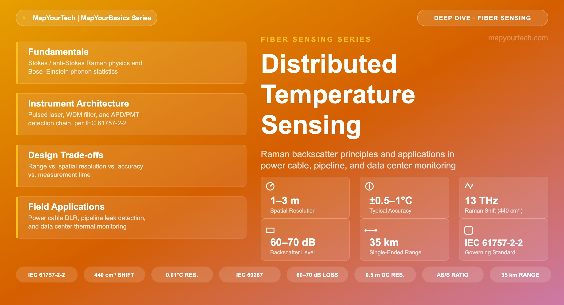
A much smaller fraction of the returning light has exchanged energy with the vibrational (phonon) modes of the silica lattice. This is spontaneous Raman scattering, and it appears as two symmetric sidebands around the Rayleigh peak: a longer-wavelength Stokes band, where the scattered photon has given up energy to create a phonon, and a shorter-wavelength anti-Stokes band, where the scattered photon has gained energy by absorbing a phonon that was already present from thermal motion. For fused silica the dominant Raman band sits at a frequency shift of roughly 440 cm−1 (about 13 THz) from the pump — the same vibrational band that defines the peak of the Raman gain spectrum exploited in distributed Raman amplifiers, discussed in MapYourTech's explanation of how a Raman amplifier works. DTS instruments typically place their Stokes and anti-Stokes detection bands roughly 100 nm to either side of the probe wavelength — for a 1550 nm probe, filters centered near 1450 nm (anti-Stokes) and 1650 nm (anti-Stokes/Stokes pair) are a common configuration — chosen for practical filter isolation rather than to sit exactly on the 13 THz gain peak.
The anti-Stokes photon population is the thermometer
Whether a phonon is available to be absorbed — the event that produces an anti-Stokes photon — depends on how many vibrational modes are thermally populated at that instant. That population follows Bose–Einstein statistics. The mean phonon occupation number of a vibrational mode of frequency Ω at absolute temperature T is:
This is not a DTS-specific approximation; it is the same phonon statistics that governs the noise floor of distributed Raman amplifiers, where the same asymmetry between Stokes and anti-Stokes sidebands sets the temperature-dependent noise figure of the amplifier. In a sensing context, the practical consequence is that the anti-Stokes band grows measurably brighter as the fiber warms, while the Stokes band stays comparatively stable — making the Stokes band a convenient, nearly temperature-independent reference against which to measure the anti-Stokes response.
From intensity ratio to temperature
A DTS instrument measures the intensities of the returning anti-Stokes and Stokes bands at every range bin along the fiber and takes their ratio. Because both bands originate from the same scattering event at the same location, most systematic effects — pulse energy fluctuations, coupling loss at the connector — cancel in the ratio, leaving temperature as the dominant remaining variable. Combining the Bose–Einstein population factor with the ν4 scattering-cross-section dependence common to both Raman and Rayleigh scattering gives the working demodulation equation:
Two demodulation strategies are used in practice. The dual-demodulation principle (DDP) uses the full anti-Stokes/Stokes ratio shown above, which cancels most wavelength-independent losses but remains sensitive to the differential attenuation between the two bands. The self-demodulation principle (SDP) uses only the anti-Stokes trace referenced against a stored baseline, which is simpler but more exposed to drift in launch power over time. Commercial instruments typically default to a form of DDP with attenuation compensation, and offer a loop or double-ended configuration as an option for routes where the highest accuracy is required.
Takeaway: The temperature signal in Raman DTS comes from the thermal population of phonon modes in the silica lattice, not from any property engineered into the fiber. Every standard telecom fiber is already a Raman thermometer; the instrument is what turns the effect into a calibrated, distance-resolved measurement.
3. Technical Architecture of a Raman DTS Instrument
A Raman DTS interrogator combines a pulsed laser source, a wavelength-selective optical front end, two sensitive photoreceivers, and a signal-processing chain that converts time-of-flight into distance and intensity ratio into temperature. The building blocks are conceptually close to a standard OTDR — both instruments time the return of backscattered light — but a DTS unit adds wavelength discrimination that a loss-measuring OTDR does not need.
Pulsed laser source and pulse width
The source is typically a semiconductor laser diode operating near 1550 nm (some systems use 1064 nm for shorter-range, higher-sensitivity applications), driven to produce narrow pulses at a repetition rate set by the fiber's round-trip time. Pulse width sets spatial resolution directly, since the instrument cannot distinguish two scattering events that arrive at the detector closer together than the pulse duration allows.
Wavelength filtering and photoreceivers
A wavelength-division filter, typically a dielectric thin-film or fiber Bragg grating design, separates the returning light into Stokes and anti-Stokes paths before it reaches the detectors. Each path terminates in an avalanche photodiode (APD) or photomultiplier tube (PMT) selected for high sensitivity in a signal regime that measured research places at roughly 60 to 70 dB below the launched pulse power — the dominant constraint on achievable signal-to-noise ratio in any Raman DTS design. Some commercial instruments use a single shared receiver switched between the two wavelength bands rather than two separate detectors, a design choice vendors report improves relative amplitude stability between the Stokes and anti-Stokes measurements because both signals pass through identical receiver electronics.
Reference sections and differential attenuation correction
Because anti-Stokes light attenuates faster along the fiber than Stokes light (shorter wavelengths generally see higher loss in silica), the raw intensity ratio drifts with distance even at constant temperature. Instruments handle this in one of two ways: a single-ended measurement anchored by a factory-measured attenuation profile and a known-temperature reference coil near the instrument, or a double-ended loop measurement that accesses the fiber from both ends and combines the two traces to cancel the distance-dependent attenuation term entirely, at the cost of routing two fiber connections to the far end of the route. IEC 61757-2-2, the governing test-method standard for fiber optic distributed temperature sensing, explicitly defines both the single-ended and loop configurations and specifies how each performance parameter should be measured and reported.
Takeaway: Every component in a Raman DTS instrument exists to solve one problem: extract a small, distance-dependent intensity ratio from a signal that is tens of decibels weaker than the pulse that created it, without letting attenuation, connector loss, or launch power drift masquerade as a temperature change.
4. Design Considerations: Range, Resolution, and Accuracy Trade-offs
Every Raman DTS specification sheet is a negotiation between four numbers: sensing range, spatial resolution, temperature accuracy, and measurement time. Pushing any one of them favorably costs performance in at least one of the others, and the underlying reason is always signal-to-noise ratio.
Why the trade-offs exist
Longer range means more fiber loss between the hot spot and the instrument, which weakens the returning signal at long distances. Finer spatial resolution means a narrower pulse, which puts less energy into each resolvable segment of fiber and correspondingly less signal into each detected range bin. Both effects can be offset by averaging more pulses, which improves the signal-to-noise ratio roughly with the square root of the number of averaged traces — but that directly trades against measurement time, so a system that reports temperature every second cannot match the accuracy of the same hardware averaging for several minutes.
Published research results make this trade-off concrete. Across independent studies, the pattern is consistent: shorter range and longer averaging buy tighter accuracy at fine spatial resolution, while longer range or faster updates cost accuracy at a given resolution.
Chart data (range in km, spatial resolution in m, reported accuracy, averaging time): Yang et al. 2021 single-mode RGF (2.9, 3, ±0.5°C, 15 s); early 20 km benchmark cited in Feng et al. 2022 review (20, 3, ±6°C, 80 s); Liu et al. 2018 graded-index few-mode fiber (25, 1.13, ±1°C, 90 s); Feng et al. 2022 low-water-peak fiber with denoising neural network (24, 1, ±1.77°C, 1 s).
Techniques used to push the envelope
- Pulse coding: launching coded sequences of pulses (Simplex or Golay codes) instead of single pulses, then decoding the composite return, which improves signal-to-noise ratio without lengthening the effective pulse and sacrificing resolution.
- Denoising algorithms: post-processing techniques, increasingly neural-network based as of 2026, that recover accuracy from noisier raw traces without adding acquisition time — the low-water-peak fiber result in Figure 3 combines this with a purpose-built fiber to reach 1°C-class accuracy at 1 m resolution over 24 km in a single second of averaging.
- Specialty fiber: graded-index few-mode fiber and enhanced-backscatter fiber increase the fraction of light captured per scattering event, directly raising the signal floor available to the detector.
- Loop and dual-ended configurations: beyond correcting differential attenuation, combining forward and reverse traces effectively doubles the averaged data available at each point, improving accuracy at the cost of a second fiber connection at the far end.
Design note: Specification sheets typically quote spatial resolution and temperature resolution at the shortest supported range, then relax both figures step by step as range extends — visible directly in vendor data, where a system's finest published spatial resolution is tied to its shortest range band and its coarsest resolution to its longest.
Takeaway: There is no such thing as a DTS system that is simultaneously long-range, fast, and centimeter-precise. Any two of those three properties can be optimized; the third is what pays for it, and system selection starts by deciding which one the application can afford to give up.
5. Implementation: Cable Choice, Deployment, and Calibration
Sensing cable selection
The fiber itself rarely needs to be special-purpose — standard single-mode fiber works for ranges beyond roughly 10–40 km, while multimode fiber offers stronger backscatter and is often preferred for shorter ranges up to a few tens of kilometers where its higher attenuation is not yet limiting. What does matter is the surrounding cable construction: for burial or submersion, the sensing fiber needs a jacket and armor rated for the mechanical and chemical environment of the installation, and for temperatures above roughly 100°C — found near some pipeline or process equipment — specialized high-temperature coatings and connectors replace the standard telecom-grade jacket.
Placement relative to the asset being monitored
Where the fiber sits relative to the heat source materially changes what the DTS trace represents. For an underground power cable, placing the sensing fiber inside the cable's metallic screen or neutral layer gives the closest approximation to actual conductor temperature, at the cost of complexity at every joint and termination where the screen is interrupted; placing it in a separate conduit alongside the cable is simpler to install and maintain but requires a larger thermal correction to estimate conductor temperature from the measured ambient-adjacent value. Either way, the DTS reading is a fiber-jacket temperature, not the conductor temperature directly — getting from one to the other is a calculation, not a direct reading.
Converting fiber temperature to asset temperature
For power cables, that calculation follows the Neher-McGrath thermal-resistance method formalized in IEC 60287 (electric cables — calculation of the current rating) and IEEE Std 835 (power cable ampacity tables). The method treats the path from conductor to fiber as a series of thermal resistances — conductor to insulation, insulation to sheath, sheath to soil or duct — and uses the known load current together with the measured fiber temperature to back-calculate conductor temperature and, from that, the safe continuous or emergency current rating (ampacity) at that moment. Screen-embedded fiber placement is commonly cited as achieving ±1–2°C accuracy against actual conductor temperature once this correction is applied, versus a wider margin for conduit-mounted fiber.
Calibration and validation
Commercial DTS instruments ship factory-calibrated against traceable temperature references, but field practice adds two more steps: verifying the reference coil or loop-back configuration against a known temperature at commissioning, and periodically cross-checking the distributed trace against a small number of independent point sensors (RTDs or thermocouples) co-located at accessible points along the route. This cross-validation step is not cosmetic — a recent data center thermal-monitoring study cross-validated its distributed fiber system against 30 Class A RTDs (±0.15°C accuracy) over a 72-hour period before trusting the fiber data for control decisions, and scheduled recalibration whenever drift exceeded ±0.2°C at any of ten reference points — a discipline worth adopting on any DTS deployment feeding automated control or protection logic.
Takeaway: A DTS trace is only as trustworthy as the calibration and placement decisions made before commissioning. The instrument measures fiber temperature with genuine precision; converting that into a conductor temperature, a pipeline wall temperature, or a rack-inlet temperature is an engineering calculation layered on top, and it is where most field accuracy is won or lost.
6. Performance and System Comparison
Commercial Raman and Brillouin-based DTS systems span a wide performance range, and vendors typically publish several product tiers rather than one fixed specification. The table below draws figures directly from current vendor documentation, each labeled as a vendor claim rather than an independently verified measurement.
| System | Scattering Mechanism | Sensing Range | Best Spatial Resolution | Best Temperature Resolution |
|---|---|---|---|---|
| Silixa ULTIMA-M | Raman | 2 / 5 / 10 km bands | 0.65 m | 0.01°C |
| Silixa ULTIMA-L | Raman | 10 / 20 / 35 km bands | 2.1 m | 0.03°C |
| AP Sensing DTS N62-Series | Brillouin | 80 km and beyond | Meter-class (vendor states "high spatial resolution," precise figure not published) | — |
| Bandweaver T-Laser DTS | Raman | Tens of km, typical industrial class | 1 m | 0.01°C sensing resolution, ±1°C accuracy |
Chart data (system, max range in km, best spatial resolution in m): Silixa ULTIMA-M (10, 0.65); Silixa ULTIMA-L (35, 2.1); typical industrial-class Raman DTS reported across multiple independent vendor sources (30, 1.0).
The article's own performance envelope — roughly 1–3 m spatial resolution and ±0.5°C accuracy — sits squarely inside this commercial range: finer than a long-haul, tens-of-kilometers industrial system, coarser than the shortest-range, highest-precision product tiers, and broadly consistent with what utilities and pipeline operators deploy for routine hot-spot and leak monitoring rather than research-grade characterization.
Takeaway: When comparing DTS systems, always check which range band a quoted spatial or temperature resolution applies to. A single system model can carry several published resolution figures depending on how far down the fiber it is being asked to see.
7. Applications
Three application domains account for the overwhelming majority of commercial Raman DTS deployments as of 2026: electric utility cable monitoring, oil and gas pipeline integrity, and data center thermal management. Each stresses a different corner of the range–resolution–accuracy trade-off described in Section 4.
7.1 Power Cable Monitoring and Dynamic Line Rating
Underground and submarine power cables are conservatively rated at design time against a worst-case combination of soil thermal resistivity, ambient temperature, and burial depth that rarely occurs in practice along the entire route simultaneously. A DTS trace along the cable route replaces that worst-case assumption with a real-time measurement, feeding a Real-Time Thermal Rating (RTTR) calculation that can safely raise ampacity above the static nameplate value whenever actual thermal conditions allow it, and flag the exact location of a developing hot spot before it becomes a fault.
An IEEE-documented case study on a 230 kV, 500 MVA cable circuit combined finite-element modeling with gradient-based optimization to estimate soil thermal parameters directly from DTS-recorded temperature history and load data, then used those parameters to compute validated continuous and emergency ratings for the circuit — the kind of route-specific ampacity assessment that a static IEC 60287 calculation, using generic soil assumptions, cannot provide. In a separate deployment, an Australian distribution operator installed DTS across four 33 kV underground cables covering a 20 km circuit length specifically to gain hotspot identification and bottleneck visibility that point sensors could not deliver across the full route.
Submarine and offshore export cables extend the same principle to a harder environment. As offshore wind capacity has expanded, grid operators have paired DTS for hot-spot detection with Distributed Acoustic Sensing (DAS) for third-party intrusion and fault detection on the same fiber pair — an architecture documented in 2026 case studies covering offshore wind export cable links, where the DTS channel additionally supports a Depth-of-Burial-State assessment that infers whether a cable section has become exposed on the seabed from its thermal response to load. This kind of multi-modal fiber sensing on submarine assets is a natural extension of the live monitoring techniques described in MapYourTech's coverage of live C-OTDR repeater loop integration for telecom submarine systems.
Practical Example — Real-time rating on a 230 kV circuit: A utility engineer receives a DTS trace showing the hottest 50 m segment of a 230 kV, 500 MVA underground circuit running consistently 4°C above the route average during a summer load peak. Rather than de-rating the entire circuit to protect that one segment — the conservative static-rating response — the engineer uses the DTS-derived local soil thermal resistance, combined with real-time load data per the IEEE-documented finite-element approach, to confirm the segment still has margin under IEC 60287 assumptions and issues an emergency rating increase for a defined multi-hour window instead of a blanket capacity restriction.
7.2 Pipeline Leak Detection
A pipeline leak changes the local temperature of the surrounding soil or air in a way that depends on what is leaking: escaping high-pressure gas cools the surrounding area through Joule-Thomson expansion, while a liquid product leak — crude oil extracted at above-ambient temperature is a common case — warms the surrounding soil as it exchanges heat with its new environment. A DTS cable run alongside or beneath the pipeline detects either signature as a localized deviation from the temperature trend along the rest of the route.
Field deployments illustrate both the value and the limits of temperature-only leak detection. UAE gas transmission operator GASCO introduced distributed fiber sensing on its Habshan-Ruwais-Shuweihat and Habshan-Maqta-Tawelah gas pipeline routes specifically for leak and third-party-intrusion monitoring, using a Brillouin-based distributed sensing configuration that extracts temperature information alongside strain data from the same fiber — illustrating that pipeline operators frequently choose Brillouin scattering over pure Raman DTS specifically to gain that combined temperature-and-strain capability over very long single-ended reaches, a comparison developed further in Section 8. Because ambient temperature fluctuation can mask a genuine leak signature in temperature-only data, current pipeline leak detection practice increasingly fuses DTS or Brillouin temperature data with Distributed Acoustic Sensing (DAS) vibration data from the same or a companion fiber, using the two signals' complementary strengths to separate real leak events from background noise — the sensing-technology comparison developed in MapYourTech's comparison of φ-OTDR and DAS for cable monitoring applies directly to this fusion approach.
Detection sensitivity depends heavily on burial geometry. Simulation work modeling gas pipeline leaks combined with the Raman scattering demodulation principle found that leak-induced temperature changes are detectable within roughly 100 mm of the leak point itself, with the rate and magnitude of the temperature change scaling with pipeline pressure, leak-hole size, and soil porosity — underscoring that DTS cable placement relative to the pipe wall, not just instrument sensitivity, determines real-world detection performance.
Practical Example — Distinguishing a leak from a hot day: A pipeline operator's DTS trace shows a 2°C localized cooling event at kilometer marker 47 on a gas transmission line during a period of stable ambient temperature elsewhere along the route. Because the DTS trace alone cannot rule out a local soil-moisture or burial-depth anomaly unrelated to a leak, the operator's leak-detection software cross-references a co-located DAS channel for the acoustic signature expected from escaping high-pressure gas before dispatching a field crew — the fused decision path recommended by current pipeline leak-detection selection guidance.
7.3 Data Center Thermal Monitoring
Point sensors — typically RTDs at rack inlets and computer room air conditioner (CRAC) return-air outlets — leave most of a data hall thermally unmeasured, and a hot spot forming between sensor locations goes undetected until it shows up as a hardware fault or a thermal shutdown. Routing a DTS sensing cable along the tops of cold and hot aisles and through key heat-exchange zones converts that sparse point-sensor map into a continuous thermal profile of the entire room, at spatial resolution fine enough to resolve individual rack rows rather than zone averages.
A 2026 controlled study of this approach deployed roughly 1,800 m of sensing fiber along cold- and hot-aisle tops and key heat-exchange regions in an active data hall, collecting temperature from more than 3,600 sensing points at 0.5 m spatial resolution — more than twenty times the point count of the facility's existing 156-sensor PT100 baseline. The fiber system was cross-validated against 30 co-located Class A PT100 sensors (±0.15°C accuracy) over a 72-hour period before being trusted to drive a model-predictive cooling-control loop, with weekly spot checks against ten reference points and full recalibration triggered whenever drift exceeded ±0.2°C. The resulting thermal-symmetry control approach used the dense distributed data to balance cooling delivery across aisles in real time rather than reacting to the handful of point sensors nearest the CRAC units.
Beyond hot-spot detection, the same cable run supports fire-detection duty when routed through cable trays and above suspended ceilings, and gives facility operators a long-term temperature-trend record per rack row that supports predictive maintenance decisions — identifying gradually degrading airflow or filter conditions before they become an acute thermal event, extending existing distributed sensing techniques for structures like cable tunnels and conveyor systems into the data hall itself.
Practical Example — Finding a hot spot between sensors: A facility's 0.5 m-resolution DTS trace along a hot aisle shows a 3°C localized rise centered between two rack rows that carry no dedicated point sensor at that exact position. Cross-checked against the co-located Class A PT100 network per the facility's validation protocol, the anomaly is confirmed as a genuine thermal event rather than fiber-system noise, and traced to a partially blocked perforated floor tile restricting cold-aisle airflow to that specific row — a fault invisible to the facility's original 156-sensor point network, which had no sensor positioned between the two racks in question.
Takeaway: Across all three applications, DTS earns its cost not by replacing point sensors outright but by filling the gaps between them — the segment of cable route, pipeline, or data hall floor that a discrete sensor network was never dense enough to cover in the first place.
8. Comparison with Alternative Sensing Technologies
Raman scattering is one of three backscatter mechanisms IEC 61757 recognizes for distributed fiber sensing, alongside Brillouin and Rayleigh scattering, each suited to a different combination of measurand, range, and resolution.
| Technology | Scattering Mechanism | Measurand | Typical Range | Typical Spatial Resolution |
|---|---|---|---|---|
| Raman DTS | Spontaneous Raman | Temperature only | Up to ≈10–40 km single-ended | ≈1–3 m |
| Brillouin DTS / BOTDA | Stimulated or spontaneous Brillouin | Temperature and strain (jointly) | Up to ≈80–100 km class | Meter-class, configuration-dependent |
| Rayleigh DAS / φ-OTDR | Coherent Rayleigh (phase) | Vibration / acoustic strain, not temperature | Up to ≈40–50 km, extendable with repeater access | Meter-class, gauge-length dependent |
| FBG point / quasi-distributed | Bragg reflection at discrete gratings | Temperature or strain at grating locations | Discrete points along a fiber run | Centimeter-scale at each grating |
The practical consequence for system selection: Raman DTS is the default choice when the requirement is genuinely continuous temperature coverage at moderate range and moderate cost. Brillouin systems earn their added complexity when a route needs both temperature and mechanical strain from a single fiber, or when single-ended reach beyond what Raman comfortably supports is required — the GASCO pipeline deployment discussed in Section 7.2 is exactly this case. Rayleigh-based DAS answers a different question entirely: it detects vibration and acoustic events, not temperature, and is typically deployed alongside rather than instead of a temperature-sensing channel when a route needs both capabilities, as in the offshore wind cable case in Section 7.1. FBG sensors trade distributed coverage for high accuracy at a small number of known, critical points — useful for validating a distributed system's readings rather than replacing it.
Takeaway: The choice between Raman, Brillouin, and Rayleigh-based sensing is rarely about which is "better" in the abstract. It follows directly from whether the application needs temperature, strain, acoustic events, or some combination, and how far the fiber has to reach to deliver it.
9. Future Directions
Three trends are shaping where Raman DTS deployment is headed through the rest of this decade. First, machine-learning-based denoising is moving from research demonstration to production instrument firmware — the low-water-peak-fiber result in Figure 3, which reached 1°C-class accuracy at 1 m resolution over 24 km with only one second of averaging, depended as much on its denoising neural network as on the specialty fiber itself, and that pattern of software-driven performance gains on existing hardware is likely to continue.
Second, multi-modal fiber sensing — combining DTS with DAS, state-of-polarization (SOP) monitoring, and even coherent-transceiver-derived sensing on the same cable — is becoming the default architecture for critical infrastructure rather than an experimental add-on. A 2026 OFC technical paper demonstrated combined distributed acoustic, state-of-polarization, and Brillouin sensing on a 118 km subsea cable, capturing storm-induced strain events with distinct signatures across each modality, and industry group CIGRE has scheduled dedicated sessions on distributed fiber optic sensing for underground and submarine power cables at its Paris Session in August 2026 — a signal that utilities are formalizing this multi-parameter approach into standard practice rather than treating it as a pilot technology. This trend extends naturally from developments in submarine telecom cable sensing, including the live monitoring architectures covered in MapYourTech's guide to undersea repeater systems and the broader system design questions explored in MapYourTech's analysis of the submarine cable stack.
Third, the economic case for adding sensing capability to power infrastructure is strengthening independently of sensor cost, because offshore wind cable failures alone are reported in recent research as accounting for a large share of total financial losses across offshore wind projects — making early thermal and mechanical fault detection a direct driver of project economics rather than a compliance afterthought. As dynamic line rating and real-time thermal rating become standard utility practice rather than a differentiator, expect the DTS instrument itself to keep converging toward being one channel in a shared multi-parameter interrogator rather than a dedicated single-purpose box.
Takeaway: The physics of Raman backscatter thermometry has not changed in decades; what is changing is how much of a system's performance now comes from signal processing rather than optics, and how routinely temperature sensing gets bundled with acoustic and strain sensing on the same strand of glass.
Related Articles on MapYourTech