

Generic selectors
Exact matches only
Search in title
Search in content
Post Type Selectors
Articles
lp_course
lp_lesson
Back
HomeCoherent OpticsGeneralized OSNR (GOSNR): Beyond Traditional OSNR
Generalized OSNR (GOSNR): Beyond Traditional OSNR

Generalized OSNR (GOSNR): Beyond Traditional OSNR

Last Updated: April 2, 2026
31 min read
86
Generalized OSNR (GOSNR): Beyond Traditional OSNR | MapYourTech
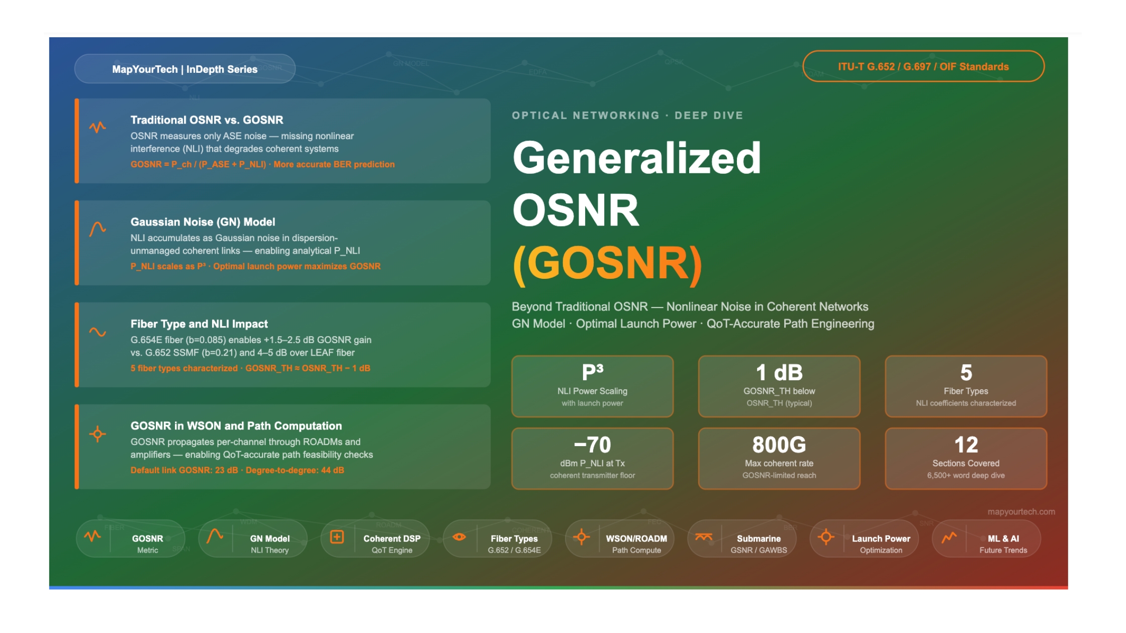
Generalized OSNR (GOSNR): Beyond Traditional OSNR - Image 1

Generalized OSNR (GOSNR): Beyond Traditional OSNR

How the GN Model and Nonlinear Interference Noise Transform System Performance Prediction in Dispersion-Unmanaged Coherent Networks

1. Introduction

Optical signal-to-noise ratio (OSNR) has been the primary engineering metric in optical transport networks for decades. It quantifies the ratio of signal power to accumulated amplified spontaneous emission (ASE) noise, measured by an optical spectrum analyzer across a 0.1 nm reference bandwidth. For the intensity-modulated, directly detected systems that preceded coherent technology, this linear OSNR was an excellent proxy for system performance. Feed the right number into a BER formula, and you knew whether your link would work.

Coherent transmission changed the rules. When dispersion-managed systems gave way to dispersion-unmanaged coherent architectures — where chromatic dispersion compensation fiber (DCF) was removed from the link, replaced by electronic dispersion compensation in the transceiver's DSP — a new class of impairment emerged as a first-order concern. Fiber nonlinearity, particularly the Kerr effect, began generating noise that could no longer be separated cleanly from ASE by the receiver. In a well-dispersed link where signals rapidly spread spectrally, the nonlinear interaction products accumulate in a statistically Gaussian manner, indistinguishable from amplifier noise to the coherent DSP. Traditional OSNR, which accounts only for ASE, began to overestimate system performance.

This created an engineering gap. Designers working with 100G coherent QPSK over legacy terrestrial infrastructure saw OSNR values that looked healthy on the optical spectrum analyzer but still experienced BER degradation at high launch powers. The explanation lay in nonlinear interference (NLI) noise — a power-dependent noise contribution invisible to the OSA's linear noise model.

Generalized OSNR (GOSNR) addresses this gap. It extends the traditional OSNR definition to include NLI noise as an additional noise term in the denominator, alongside ASE. The result is a single metric that captures the true noise environment seen by the coherent receiver, enabling more accurate reach prediction, more precise power optimization, and more reliable quality-of-transmission (QoT) estimation in automated network management systems. This article presents the physical foundations, mathematical structure, and practical applications of GOSNR in modern dispersion-unmanaged optical networks.

2 Noise Terms in GOSNR
(ASE + NLI)
~1 dB Typical GOSNR vs OSNR gap at optimal launch power
3 dB Typical NLI impact at +3 dBm above optimum power
P3 NLI noise power scaling with channel launch power

2. Historical Evolution: From Linear to Generalized SNR

2.1 The Linear OSNR Era

The concept of OSNR emerged with wavelength-division multiplexing (WDM) in the 1990s, when the industry needed a simple, measurable figure of merit for multi-span amplified links. The ITU-T formalized OSNR measurement methodology in Recommendation G.697 (Optical monitoring for DWDM systems), which specified the 0.1 nm reference bandwidth and the interpolation-based noise floor measurement using an optical spectrum analyzer. For intensity-modulated direct-detection (IMDD) systems running at 2.5 Gbps and 10 Gbps, this approach was highly accurate because nonlinear effects were either weak (low symbol rate, lower power densities) or handled through careful dispersion management that broke up nonlinear phase accumulation.

The 40 Gbps generation revealed early signs of the limitation. At this bit rate, launch powers needed to maintain adequate OSNR started pushing systems toward nonlinear regimes, and dispersion management itself introduced nonlinear phase matching conditions that made FWM and XPM significant impairments. Engineers compensated with careful span-by-span power control and exact dispersion map design, but the system design process grew complex and the linear OSNR metric began to require empirical correction factors.

2.2 Coherent Transmission and the Nonlinear Noise Problem

The industry transition to coherent 100G PDM-QPSK around 2010–2012 fundamentally altered the noise landscape. These systems removed DCF from the line, relying entirely on the coherent receiver's DSP to compensate for accumulated chromatic dispersion. This created dispersion-unmanaged links where the optical signal was in a heavily dispersed state for most of its propagation. The key insight — confirmed by extensive simulation and analytical work — was that in such links, the nonlinear interaction products adopt a Gaussian statistical distribution by the time they reach the receiver, thanks to the averaging effect of strong dispersive mixing among WDM channels over long distances.

This is the physical regime in which the Gaussian Noise (GN) model, developed analytically between 2010 and 2013 by multiple research groups, applies. The GN model predicts that in dispersion-unmanaged multi-channel coherent systems, the NLI noise power spectral density can be computed analytically as a function of signal power, fiber parameters, and system configuration. It behaves as additive white Gaussian noise — the same statistical character as ASE. This meant NLI and ASE could be summed in the noise denominator using the same mathematical framework, producing GOSNR.

Why Gaussian Noise Behavior Matters

In a strongly dispersed link, individual WDM channels spread rapidly in time, causing their pulses to overlap extensively with pulses from other channels. The nonlinear interaction at any point in the fiber involves a large number of effectively random symbol combinations. By the central limit theorem, the accumulated effect approaches a Gaussian distribution. This is the physical basis for the GN model's applicability — and why GOSNR works as a single Gaussian noise budget.

2.3 The GN and EGN Models

The Gaussian noise (GN) model, as developed in the 2011–2014 timeframe, predicts NLI power as a function of channel power, fiber nonlinear coefficient, dispersion, span length, and WDM comb parameters. The GN model uses a signal Gaussianity approximation — treating the WDM signal as if it were Gaussian-distributed. This provides an upper bound on NLI: real PM-QAM signals, being non-Gaussian in their symbol statistics, generate slightly less NLI than the GN model predicts.

The extended GN model (EGN model) corrects for this by adding a negative correction term that accounts for the non-Gaussian statistical features of the actual modulation format. For PM-QPSK, the EGN correction is small at typical system lengths. For PM-16QAM and higher-order formats, the correction becomes more significant, and the EGN model provides materially better accuracy. Both models confirm that NLI noise power scales approximately as the cube of per-channel launch power (P³), which has profound implications for link optimization.

3. Fundamental Principles of GOSNR

3.1 The GOSNR Definition

Traditional OSNR is defined as the ratio of signal channel power Pch to ASE noise power PASE, typically referenced to a 0.1 nm bandwidth. GOSNR extends this by adding the nonlinear interference noise power PNLI to the noise denominator:

Equation 3.1 — GOSNR Definition (Linear Power)
GOSNR = P_ch / ( P_ASE + P_NLI )

In logarithmic (dB) form:

GOSNR(dB) = P_ch(dBm) - 10·log₁₀[ P_ASE,lin + P_NLI,lin ]

Where P_ASE,lin = 10^(P_ASE/10) in mW
      P_NLI,lin = 10^(P_NLI/10) in mW
P_chChannel signal power at the measurement port (dBm or mW)
P_ASEAccumulated ASE noise power from optical amplifiers (dBm or mW)
P_NLINonlinear interference noise power generated in transmission fiber (dBm or mW)
GOSNRGeneralized optical signal-to-noise ratio (dimensionless or dB)

Note that when PNLI is negligible — as in short links, low-power systems, or dispersion-managed networks — GOSNR converges to the traditional OSNR. The two metrics diverge as launch power increases and PNLI grows toward the magnitude of PASE.

3.2 The Inverse SNR Summation Principle

A more general formulation of GOSNR follows directly from the principle that independent Gaussian noise sources can be combined by summing their inverse SNR contributions. When all sources of signal impairment can be modeled as Gaussian — ASE noise, nonlinear interference, GAWBS (guided acoustic wave Brillouin scattering) in submarine systems, and other effects — the aggregate inverse SNR equals the sum of individual inverse SNRs:

Premium Article — Free 21% Preview

Read the Full Analysis with Premium

The remaining 79% of this article — the design numbers, trade-offs and field guidance — is part of MapYourTech Premium, along with the full premium library, courses and professional tools.


Instant access · Cancel anytime · 48-hour trial available
Sanjay Yadav

Optical Communications & Network Automation Expert | Author of 3 Books for Optical Engineers | Founder, MapYourTech

Optical networking engineer with nearly two decades of experience across DWDM, OTN, coherent optics, submarine systems, and cloud infrastructure. Founder of MapYourTech.

Follow on LinkedIn

You May Also Like

52 min read 12 0 Like The Submarine Cable Stack: Open Cables, GSNR, SDM and Power Skip to main content...
  • Free
  • July 10, 2026
32 min read 10 0 Like Coherent DSP Architecture: From ADC Samples to Client Bits MAPYOURTECH | COHERENT OPTICS DEEP...
  • Free
  • July 10, 2026
42 min read 14 0 Like Building an Optical NOC Dashboard with OpenConfig Telemetry Skip to main content MapYourTech |...
  • Free
  • July 10, 2026

Course Title

Course description and key highlights

Course Content

Course Details
