
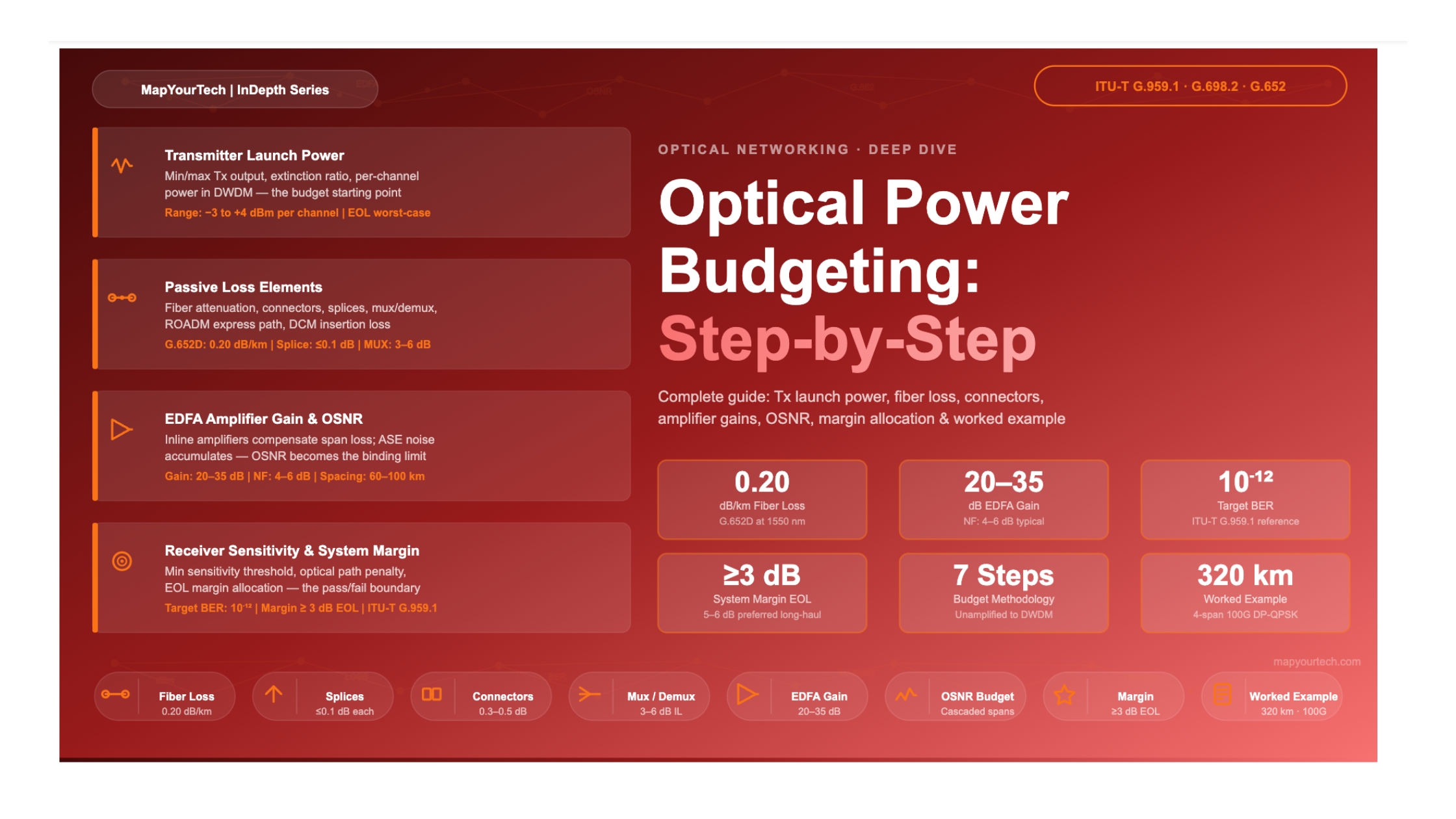

Optical Power Budgeting: Step-by-Step Guide
1 Introduction
Why every optical link starts with a power budget
An optical power budget is the systematic accounting of signal power available in a transmission link, weighed against every source of loss, from the first connector on the transmitter shelf to the final detector at the receiver. Done correctly, it tells you whether a link will work — and by how much margin — before a single fiber is pulled through conduit.
The concept is deceptively simple: a transmitter emits light at a known power level, that power attenuates as it travels through fiber, connectors, splices, multiplexers, amplifiers, and add/drop nodes, and the residual power must exceed the receiver's minimum sensitivity threshold by a comfortable margin. The complexity arises in rigorously quantifying every element of that journey, accounting for worst-case tolerances, end-of-life degradation, and the subtle penalties imposed by dispersion, polarization effects, and optical noise from amplifiers.
In unamplified (passive) systems, the power budget is governed primarily by the difference between transmitter output power and receiver sensitivity, with all attenuation sources sitting between them. In amplified long-haul and DWDM systems, as described in ITU-T Recommendation G.698.2, the dominant limit shifts from raw optical power to Optical Signal-to-Noise Ratio (OSNR), which accumulates with every amplifier stage. Both regimes demand the same foundational skill: the ability to enumerate, quantify, and sum every contributor to signal degradation.
For unamplified systems: Minimum Tx power − Minimum Rx sensitivity > Maximum link attenuation + Maximum optical path penalty (ITU-T G.959.1). For amplified systems, the equivalent inequality is expressed in OSNR.
This guide walks through each element of the power budget in logical order — transmitter characteristics, every category of passive loss, amplifier gains, OSNR considerations, margin allocation, and a complete worked example spanning a 320 km DWDM link with inline EDFA amplification. The approach follows worst-case, end-of-life (EOL) design methodology, consistent with ITU-T practice, which ensures that a link designed to specification will remain within tolerance throughout its operational lifetime.
2 Fundamental Principles
The mathematics of optical power in dB and dBm
2.1 Working in dB and dBm
All optical power budget calculations are performed in logarithmic units. Power levels are expressed in dBm (decibels relative to 1 milliwatt) and losses or gains are expressed in dB. This convention transforms the product of multiple gain and loss factors into a simple sum — an enormous practical advantage when a link contains dozens of components.
PdBm = 10 × log10(PmW / 1 mW)PRx(dBm) = PTx(dBm) − Lfiber(dB) − Lconnectors(dB) − Lsplices(dB) − Lmux/demux(dB) − Lother(dB)
Pass condition: PRx(dBm) ≥ Smin(dBm) + Msystem(dB)PRx(dBm) = PTx(dBm) − ∑Llosses(dB) + ∑Gamp(dB)
Or equivalently: PRx(dBm) = PTx(dBm) + Gnet(dB)2.2 Worst-Case Design Methodology
ITU-T standards, particularly G.959.1 and G.698.2, prescribe a worst-case approach to power budget calculations. Rather than using nominal values, the design must pass using the combination of parameters that produces the worst outcome:
The transmitter is operated at its minimum guaranteed output power. Every loss element is evaluated at its maximum specified value. The receiver's minimum sensitivity threshold — not its typical sensitivity — is used as the acceptance criterion. Additionally, the optical path penalty, which captures the degradation introduced by chromatic dispersion, polarization mode dispersion (PMD), reflections, and nonlinear effects, is added on top of the minimum receiver sensitivity as an additional budget deduction.
End-of-Life (EOL) vs. Beginning-of-Life (BOL): EOL budgets add a fiber aging margin (typically 0.05 dB/km × years of operation, or a fixed 3–4 dB total aging allowance) to account for the gradual increase in fiber attenuation over the network's operational lifetime. BOL designs may appear to have large margins that will narrow over time.
Read the Full Analysis with Premium
The remaining 88% of this article — the design numbers, trade-offs and field guidance — is part of MapYourTech Premium, along with the full premium library, courses and professional tools.



Course Title
Course description and key highlights
Course Content
Course Details
Celebrating 1,000+ LinkedIn posts
3 hours of Premium Pro, free
The full Premium Pro library, unlocked with one click. The clock starts the moment you check out and runs for 3 full hours - pick a time when you can make the most of it.
- Courses
- Interview preparation content
- Career development posts
- Simulators
- Calculators
- Market research
No card, nothing to cancel. One pass per person. Sign in or create a free account at checkout.
Follow MapYourTech on LinkedIn for regular updates and future promos.
New articles, tool releases and member offers, posted as they go live.
Follow MapYourTech on LinkedIn
Enjoying MapYourTech? Follow us on LinkedIn. One click and this stops appearing.
- New technical articles and tool releases, posted as they go live
- Course launches and member offers before they reach the site
- Standards and industry updates worth an optical engineer's time
New articles, tool releases and member offers, posted as they go live.