
Limitation of Total Optical Power (TOP) in Submarine Optical Networks
Technical Guide for Optical Professionals: Understanding Power Constraints, Nonlinear Effects, and System Optimization
Introduction
Total Optical Power (TOP) limitation represents one of the most fundamental constraints in submarine optical communication systems, significantly impacting system capacity, reach, and overall performance. Unlike terrestrial systems with readily accessible power infrastructure, submarine cables face unique challenges in power delivery and management that directly influence optical transmission capabilities.
In submarine systems, the Total Output Power refers to the aggregate optical power launched into the fiber by optical amplifiers (typically Erbium-Doped Fiber Amplifiers or EDFAs) along the transmission path. This power must be carefully controlled to balance two competing requirements: maintaining sufficient signal strength for adequate Optical Signal-to-Noise Ratio (OSNR) while avoiding excessive nonlinear impairments that degrade signal quality.
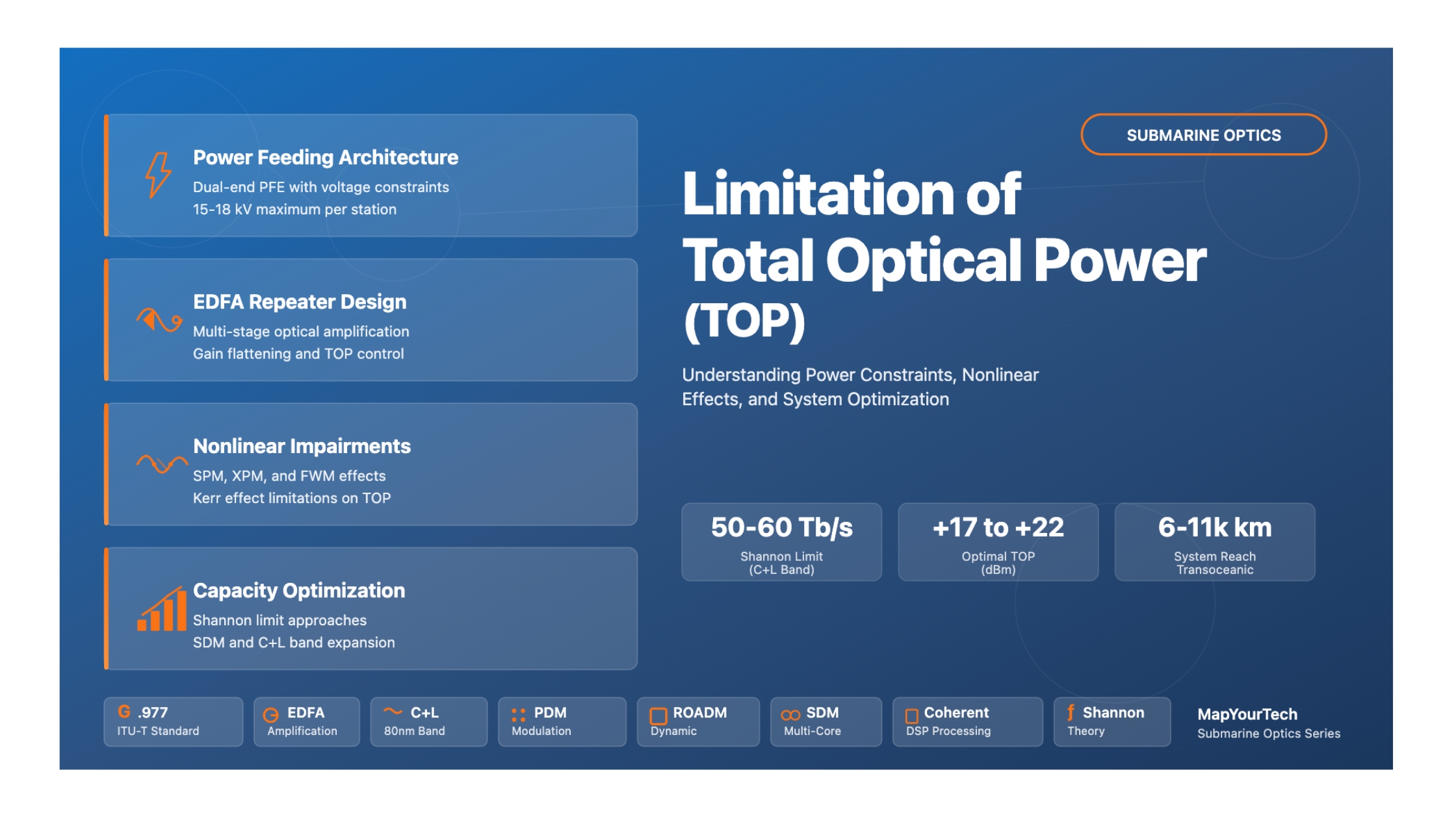
The limitation of TOP is critical because submarine systems operate under strict power feeding constraints. Power Feeding Equipment (PFE) at cable landing stations provides DC current to underwater repeaters through the cable's inner conductor, with return paths through seawater and earth electrodes. The maximum voltage typically ranges from 15-18 kV, limiting the total available electrical power for all repeaters across thousands of kilometers.
This comprehensive guide explores the fundamental principles, technical challenges, optimization strategies, and practical implementations related to TOP limitations in modern submarine optical networks.
Historical Context & Evolution
Technology Timeline
The evolution of submarine optical communications has been marked by progressive improvements in power management and capacity optimization. Understanding this historical progression provides context for current TOP limitations and future development directions.
Key Milestones
The journey from basic EDFA-based systems to today's sophisticated coherent, multi-band, and space-division multiplexed systems reveals continuous innovation in managing TOP constraints:
1995-2000: EDFA Revolution - The introduction of Erbium-Doped Fiber Amplifiers eliminated the need for electrical regeneration, but introduced new challenges in managing amplified spontaneous emission (ASE) noise and nonlinear effects. Early systems operated with limited TOP control, typically in C-band only.
2001-2008: Bandwidth Expansion - C+L band systems emerged, doubling the available spectrum. However, this required more sophisticated gain equalization and TOP management across wider bandwidths, pushing against fundamental power feeding limitations.
2009-2015: Coherent Era - Digital coherent technology revolutionized submarine systems, enabling electronic dispersion compensation and advanced modulation formats. This period saw the optimization of TOP to balance linear and nonlinear noise, with systems approaching Shannon limit predictions.
2016-Present: SDM and Open Systems - Space Division Multiplexing (SDM) with multi-core fibers emerged as a response to power limitations. Rather than increasing power per fiber (limited by PFE voltage constraints), capacity scales through spatial parallelism. Open cable concepts with ROADM-based terminals enable dynamic TOP optimization.
Core Concepts & Fundamentals
What is Total Optical Power (TOP)?
Total Optical Power (TOP) represents the aggregate optical power launched into the transmission fiber by an optical amplifier. In submarine systems, each repeater (containing one or more EDFAs) is designed to maintain a specific TOP level to ensure optimal transmission performance across all wavelength channels.
TOP is typically expressed in dBm (decibels relative to 1 milliwatt) and represents the sum of power across all wavelength-division multiplexed (WDM) channels plus any continuous wave (CW) idlers or amplified spontaneous emission (ASE) that may be present.
where P_i is the linear power (in mW) of each channel
The Fundamental Trade-off
The central challenge in submarine optical system design is balancing two opposing effects that both depend on optical power:
Linear Noise (ASE): Amplifiers generate ASE noise that accumulates along the transmission path. Higher TOP improves the signal-to-noise ratio by maintaining stronger signal levels relative to this noise.
Nonlinear Effects: Optical fiber exhibits intensity-dependent refractive index changes (Kerr effect), causing self-phase modulation (SPM), cross-phase modulation (XPM), and four-wave mixing (FWM). These effects worsen with higher TOP, degrading signal quality.
Key Performance Metrics
Several critical metrics govern TOP optimization in submarine systems:
Generalized OSNR (GOSNR): This metric combines both linear ASE noise and nonlinear interference noise into a single figure of merit that accurately predicts system performance. GOSNR acknowledges that in modern coherent systems, nonlinear effects manifest as noise-like impairments.
where P_NLI is nonlinear interference power
Generalized Signal-to-Noise Ratio (GSNR): Similar to GOSNR but normalized per bandwidth and used in Shannon capacity calculations. GSNR is the metric that determines achievable spectral efficiency.
Q-factor: A measurement of signal quality at the receiver, related to bit error ratio (BER). The Q-factor must exceed specified thresholds (typically corresponding to BER < 10⁻¹³ after FEC) at both beginning of life (BOL) and end of life (EOL) conditions.
Technical Architecture & Components
Power Feeding Architecture
The power feeding system is fundamental to understanding TOP limitations. Unlike terrestrial systems with ubiquitous AC power, submarine cables must deliver electrical power over thousands of kilometers to energize underwater repeaters.
Power Feeding Constraints
The power feeding system imposes several fundamental constraints on submarine cable design:
Voltage Limitations: Modern PFE systems typically operate at maximum voltages of 15-18 kV. This voltage must be shared across all repeaters in series along the cable. For a transpacific cable with ~100 repeaters, each repeater receives only ~150V if using dual-end feeding (30 kV total system voltage).
Current Constraints: PFE systems operate in constant current mode (typically 1.0-1.2 A) to ensure stable repeater operation. The current remains constant throughout the cable, with each repeater consuming power based on its voltage drop.
Total Power Budget: For a typical transpacific system with dual-end feeding at 15 kV and 1 A from each end, the total available power is 30 kW. This must power all repeaters and cover cable resistive losses.
Critical Limitation: The power feeding voltage limit directly constrains the number of repeaters that can be deployed, which in turn limits the available optical power per repeater. This creates a fundamental trade-off between system reach (requiring more repeaters with closer spacing) and per-repeater optical power budget.
EDFA Repeater Architecture
Each submarine repeater contains multiple EDFA stages to amplify the optical signals. The key components include:
Erbium-Doped Fiber (EDF): Special optical fiber doped with erbium ions that provide optical gain when pumped by 980nm or 1480nm laser diodes. The length and doping concentration are optimized for specific gain and noise figure targets.
Pump Lasers: High-power semiconductor lasers (typically 980nm for low noise figure) that excite erbium ions. The number and power of pump lasers determine the maximum achievable TOP, but are constrained by available electrical power.
Gain Flattening Filters (GFF): Optical filters that equalize gain across the C-band or C+L band spectrum. However, GFFs reduce TOP by attenuating higher-gain wavelengths, representing a trade-off between spectral flatness and total available power.
A typical submarine EDFA converts electrical power to optical power with approximately 30-40% efficiency (wall-plug efficiency). For example, 150W of electrical power might generate 50-60W of optical pump power, which produces ~18 dBm (63 mW) of total optical signal power at the output. The remaining power is dissipated as heat in the fiber and pump lasers.
Mathematical Models & Analysis
Shannon Capacity and the Shannon Limit
The theoretical maximum capacity of a submarine optical fiber is governed by Shannon's theorem, which relates channel capacity to bandwidth and signal-to-noise ratio:
where:
C = capacity per fiber pair (2 polarizations)
B = optical bandwidth (Hz)
SNR = signal-to-noise ratio (linear units)
For submarine systems, the achievable SNR is fundamentally limited by the interplay between ASE noise and nonlinear interference noise, both of which are influenced by TOP.
Gaussian Noise (GN) Model
The GN model provides an analytical framework for predicting nonlinear interference in WDM systems. It treats nonlinear effects as an additive Gaussian noise source, enabling closed-form capacity estimates.
where:
γ = fiber nonlinear coefficient (1/W/km)
L_eff = effective span length
P_ch = power per channel
N_ch = number of channels
Δf = channel spacing
This model reveals that nonlinear noise grows with the cube of channel power and the square of the number of channels, explaining why simply increasing TOP yields diminishing returns and eventually degrades performance.
Power Budget Analysis
The power budget table (PBT) is the central tool for submarine system design, accounting for all power-related parameters from beginning of life (BOL) to end of life (EOL):
| Parameter | Typical Value | Description |
|---|---|---|
| Mean Launched Power | +2 to +6 dBm/ch | Power per channel at transmitter |
| Repeater Output Power (TOP) | +17 to +22 dBm | Total power across all channels |
| Span Loss | 16-20 dB | Fiber attenuation over 80-90km |
| EDFA Gain | 16-24 dB | Amplifier gain per repeater |
| EDFA Noise Figure | 4.5-6 dB | Amplifier noise contribution |
| OSNR at Receiver (BOL) | 18-22 dB | Signal quality at system start |
| System Margin | 2-3 dB | Reserve for penalties and aging |
| Aging Allowance | 0.5-1 dB | Component degradation over 25 years |
| Repair Allowance | 1-3 dB | Additional loss from cable repairs |
Nonlinear Effects and Impairments
Kerr Effect and Intensity-Dependent Phenomena
The optical Kerr effect causes the refractive index of silica fiber to vary with optical intensity. This fundamental physical phenomenon is the source of all fiber nonlinear impairments and creates a hard limit on the maximum useful optical power.
where:
n₀ = linear refractive index (~1.45)
n₂ = nonlinear index coefficient (~2.6 × 10⁻²⁰ m²/W)
I = optical intensity (W/m²)
Impact on System Performance
Each nonlinear effect contributes differently to overall system degradation:
Self-Phase Modulation (SPM): Dominant in single-channel systems or when channels are well-separated. SPM causes spectral broadening proportional to signal intensity variations, effectively reducing spectral efficiency. In submarine systems with electronic dispersion compensation, SPM penalties can be partially mitigated through digital signal processing.
Cross-Phase Modulation (XPM): Becomes significant in dense WDM systems where multiple channels co-propagate. The intensity fluctuations of neighboring channels induce phase variations, manifesting as amplitude noise after chromatic dispersion. XPM penalties increase with channel count and power.
Four-Wave Mixing (FWM): Particularly problematic in low-dispersion or dispersion-managed systems. Three optical frequencies mix to create new frequency components at f_FWM = f_i + f_j - f_k. Modern uncompensated submarine cables with high accumulated dispersion naturally suppress FWM.
The Nonlinear Threshold: There exists a practical maximum channel power (typically +2 to +6 dBm depending on fiber type and system design) beyond which nonlinear penalties exceed linear OSNR gains. This threshold fundamentally limits how much TOP can beneficially be increased, even if electrical power were unlimited.
Optimization Strategies and Modern Solutions
Dynamic TOP Management
Modern submarine systems employ sophisticated techniques to optimize TOP throughout the cable lifetime and across varying traffic loads:
CW Idlers and ASE Loading
To maintain stable TOP in submarine repeaters regardless of traffic channel count, operators employ two key techniques:
Continuous Wave (CW) Idlers: Unmodulated optical carriers placed at specific wavelengths to "fill" the spectrum. Idlers maintain constant loading on EDFAs, preventing repeater gain changes when traffic channels are added or removed. This ensures that adding new channels doesn't perturb existing channels' nonlinear operating point.
Channelized ASE: Modern ROADM-based systems can use wavelength-selective switches to create "channel holders" - blocks of ASE noise at specific wavelengths that reserve spectrum. When a traffic channel is commissioned, its corresponding ASE block is removed and replaced, ensuring no change in total TOP or spectral distribution.
By maintaining constant TOP through idlers or ASE, operators can add new traffic channels without affecting existing services. The small perturbation (typically <0.1 dB) when swapping an ASE block for a real channel is negligible compared to adding a channel that increases total power by several dB, which would alter the nonlinear operating point for all channels.
Space Division Multiplexing (SDM)
When power-per-fiber becomes the limiting factor, SDM offers a path to continued capacity growth by increasing spatial parallelism rather than optical power:
Multi-Core Fibers (MCF): These fibers contain multiple isolated cores within a single cladding. A 7-core MCF can potentially carry 7× the capacity of a single-mode fiber using the same cable cross-section and roughly the same power budget (power is shared among cores).
Power Budget Advantage: The key benefit for TOP-constrained systems is that SDM distributes the total available optical power across multiple cores, reducing power density per core. This lowers nonlinear penalties while maintaining aggregate capacity growth. For a fixed PFE power budget, MCF enables linear capacity scaling that is otherwise impossible in single-core systems approaching the Shannon limit.
C+L Band and Bandwidth Expansion
Another path to capacity growth within TOP constraints is expanding the optical bandwidth:
C+L Band Systems: By utilizing both C-band (1530-1565 nm) and L-band (1565-1625 nm), systems nearly double their available spectrum from ~4.9 THz to ~9.8 THz. This provides a linear capacity increase proportional to bandwidth, without requiring higher per-channel power.
Wideband EDFAs: These specialized amplifiers provide gain across both C and L bands simultaneously. However, they face challenges in gain flattening across such wide bandwidth, and the need for additional gain stages may consume more electrical power from the limited PFE budget.
Raman Amplification: Distributed Raman gain uses the transmission fiber itself as the gain medium, complementing EDFAs. Raman amplification can enable even wider bandwidth (potentially 35+ THz) and improves noise performance, but requires careful TOP management to balance Raman pump power and signal power within the nonlinear threshold.
Practical Implementation & Case Studies
Real-World System Examples
Modern submarine systems demonstrate various approaches to managing TOP limitations:
Case Study 1: Transatlantic C-Band System (~6000 km)
A typical modern transatlantic cable operates with the following parameters:
| Parameter | Value | Notes |
|---|---|---|
| Cable Length | ~6000 km | US East Coast to Europe |
| Number of Repeaters | ~70-75 | ~80 km span length |
| PFE Configuration | Dual-end, 15 kV each | Total 30 kV system voltage |
| Repeater Voltage Drop | ~200 V | Per repeater at 1 A |
| Repeater Power | ~200 W | Electrical power consumption |
| TOP per Repeater | +19 dBm | ~80 mW total optical |
| Channel Count | 96 × 50 GHz | C-band spectrum |
| Per-Channel Power | +3 dBm | ~2 mW per channel |
| Modulation Format | PDM-16QAM | Modern coherent |
| Channel Bit Rate | 200-300 Gb/s | Depending on distance |
| Total Capacity | ~20-25 Tb/s | Per fiber pair |
This system operates near its optimal TOP, balancing ASE noise (dominant at lower power) and nonlinear interference (dominant at higher power). The PFE voltage constraint directly limits the number of fiber pairs that can be deployed in the cable.
Case Study 2: Transpacific C+L System (~9000 km)
Longer cables face even tighter TOP constraints due to the larger number of repeaters:
| Parameter | Value | Impact of Distance |
|---|---|---|
| Cable Length | ~9000-11000 km | US West Coast to Asia |
| Number of Repeaters | ~110-130 | More repeaters = less power each |
| Repeater Voltage Drop | ~115-130 V | Reduced to fit voltage budget |
| Repeater Power | ~115-130 W | Lower than Atlantic systems |
| TOP per Repeater | +17-18 dBm | Reduced vs. Atlantic |
| Bandwidth | C+L (~80 nm) | Essential for capacity |
| Per-Channel Power | +1 to +2 dBm | Lower to control nonlinearity |
| Modulation | PDM-8QAM/16QAM | Adaptive to OSNR |
| Capacity per FP | ~15-20 Tb/s | Bandwidth compensates lower OSNR |
The transpacific case illustrates how distance exacerbates TOP limitations. With ~50% more repeaters than Atlantic systems but the same PFE voltage limit, each repeater receives proportionally less power, reducing achievable TOP. The system compensates by expanding bandwidth (C+L) rather than increasing spectral efficiency.
Troubleshooting and Optimization Guide
Common TOP-related issues and their solutions:
Problem: OSNR Degradation Over Time
Symptom: Gradual increase in BER, margin reduction. Cause: Repeater pump laser aging, fiber loss increase from hydrogen aging. Solution: (1) Implement predictive maintenance using SLTE telemetry, (2) Increase TOP slightly if power margin available, (3) Reduce modulation order or spectral efficiency to maintain margin.
Problem: Excessive Nonlinear Penalty on New Channels
Symptom: Newly added channels show worse performance than expected. Cause: Improper TOP management when adding channels increased nonlinear loading. Solution: (1) Use CW idlers or ASE loading to maintain constant TOP, (2) Reduce per-channel power slightly, (3) Implement per-channel power pre-emphasis via ROADM.
Problem: Unequal Channel Performance Across Spectrum
Symptom: Some wavelengths perform significantly worse than others. Cause: EDFA gain tilt, inadequate gain flattening. Solution: (1) Optimize GFF settings, (2) Use WSS-based per-channel equalization, (3) Adjust repeater TOP to balance gain flatness vs. total power.
Problem: Insufficient Capacity Growth Headroom
Symptom: Cannot add more channels without degrading existing services. Cause: Operating at maximum TOP limit, nonlinear threshold reached. Solution: (1) Deploy C+L band expansion if currently C-only, (2) Implement SDM with multi-core fibers for future cables, (3) Upgrade to more spectrally efficient modulation formats, (4) Add fiber pairs if cable has dark fibers.
Fiber Technology and TOP Optimization
Fiber Types and Effective Area
The choice of fiber type significantly impacts how TOP can be utilized. The effective area (A_eff) of the fiber determines the optical power density and thus the strength of nonlinear effects.
Modern submarine cables increasingly deploy G.654 type fibers (also known as Large Effective Area Fibers or LEAF) which offer:
Reduced Nonlinear Coefficient: With A_eff of 125-150 μm² compared to 80 μm² for standard SMF, the nonlinear coefficient (γ) is reduced by approximately 40-50%. Since nonlinear noise scales with γ², this translates to a 2-3 dB improvement in nonlinear tolerance.
Lower Attenuation: Premium G.654 fibers also achieve lower attenuation (~0.155-0.170 dB/km vs. ~0.180-0.190 dB/km for standard SMF), allowing longer amplifier spacing and reducing the total number of repeaters needed - which directly helps with PFE voltage constraints.
Advanced Amplifier Architectures
To optimize TOP while maintaining spectral flatness and noise performance, modern submarine systems employ sophisticated amplifier designs:
Future Technologies and Research Directions
Hollow-Core Fibers
Hollow-core fibers represent a potential paradigm shift in submarine transmission, offering fundamentally different approaches to managing TOP limitations:
Ultra-Low Nonlinearity: Since light propagates primarily in air/vacuum rather than silica, the nonlinear coefficient is reduced by approximately 1000× compared to solid-core fiber. This could potentially allow TOP levels of +25-30 dBm without significant nonlinear penalties.
Reduced Latency: Light travels at approximately 99.7% of vacuum speed of light in hollow-core fiber (compared to 68% in solid silica), providing ~30-35% latency reduction. This is valuable for financial trading and other latency-sensitive applications.
Current Challenges: Manufacturing scalability, achieving attenuation competitive with solid-core fibers (<0.15 dB/km target), and bandwidth limitations remain active research areas. Commercial submarine deployment is likely 5-10+ years away.
Advanced Modulation and DSP
Probabilistic constellation shaping (PCS) and geometric shaping techniques are enabling submarine systems to approach Shannon limits more closely, extracting maximum capacity from available TOP and OSNR budgets.
Summary and Best Practices
Design Guidelines for TOP Optimization
Based on industry experience and current best practices:
1. Early System Planning: Conduct thorough power budget analysis during the design phase. Use accurate GN model simulations accounting for actual fiber types, repeater spacing, and modulation formats. Build in adequate margin (2-3 dB minimum) for aging and repairs.
2. Fiber Selection: For new deployments, prioritize large effective area fibers (G.654) offering 2-3 dB better nonlinear performance. Consider the attenuation-nonlinearity trade-off carefully based on system length.
3. Amplifier Architecture: Implement multi-stage EDFAs with independent optimization of noise figure (first stage) and saturation power (final stage). Use gain flattening filters judiciously - balance spectral flatness against TOP reduction.
4. Channel Planning: Deploy CW idlers or channelized ASE from day one to enable plug-and-play capacity expansion. Use ROADM-based terminals for dynamic per-channel power management and automatic commissioning.
5. Bandwidth Utilization: For systems approaching Shannon limits on C-band, C+L expansion provides the most straightforward capacity scaling without increasing TOP or nonlinear penalties.
6. Future-Proofing: Consider cable designs that accommodate future fiber pair additions or multi-core fiber deployment. Ensure PFE systems can support maximum voltage (18 kV) even if initially deployed at lower voltages.
7. Monitoring and Maintenance: Implement comprehensive telemetry from SLTEs and in-line monitoring. Use predictive analytics to detect aging trends and schedule proactive maintenance before margin erosion causes outages.
8. Coherent Upgrades: When upgrading legacy cables, carefully account for the nonlinear relationship between Q and OSNR in coherent systems. Use field trials to validate power budget assumptions before full deployment.
References and Standards
ITU-T Recommendations
The following ITU-T recommendations provide normative specifications for submarine optical systems:
- ITU-T G.972: Definition of terms for optical fiber submarine cable systems
- ITU-T G.973: Characteristics of repeaterless optical fiber submarine cable systems
- ITU-T G.976: Test methods applicable to optical fiber submarine cable systems
- ITU-T G.977: Characteristics of optically amplified optical fiber submarine cable systems
- ITU-T G.977.1: Transversely compatible DWDM applications in submarine cable systems
- ITU-T G.978: Characteristics of optical fiber submarine cables
- ITU-T G.979: Characteristics of optical fiber submarine links
Key Research Papers and Industry Publications
- R.-J. Essiambre and R. W. Tkach, "Capacity Trends and Limits of Optical Communication Networks," Proceedings of the IEEE, 2012
- P. Poggiolini, "The GN Model of Fiber Non-Linear Propagation and its Applications," Journal of Lightwave Technology, 2014
- J.-X. Cai et al., "Transmission Performance of Submarine Systems," various OFC and SubOptic proceedings
- A. Pilipetskii et al., "High Capacity Submarine Transmission Systems," OFC proceedings and Submarine Networks World
- Sanjay Yadav, "Optical Network Communications:An Engineer's Perspective" . Bridge the Gap Between Theory and Practice in Optical Networking.
- Open Submarine Cable Systems eBook (Various contributors), comprehensive industry reference
Industry Resources
- SubOptic Conference Proceedings - Technical papers on submarine cable technology and deployment
- Optical Fiber Communication Conference (OFC) - Latest research in coherent transmission and fiber optics
- Submarine Telecoms Forum - Industry news and technical developments
- Ciena, Infinera, Nokia, Huawei Marine - Vendor white papers and technical documentation
Important Note: This guide represents current knowledge and best practices as of 2024-2025. Submarine cable technology continues to evolve rapidly. Always consult the latest ITU-T recommendations, vendor specifications, and peer-reviewed research for mission-critical deployments.
Developed by MapYourTech Team
For educational purposes in optical networking and submarine communication systems

Optical Communications & Network Automation Expert | Author of 3 Books for Optical Engineers | Founder, MapYourTech
Optical networking engineer with nearly two decades of experience across DWDM, OTN, coherent optics, submarine systems, and cloud infrastructure. Founder of MapYourTech. Read full bio →
Follow on LinkedIn