
Optical Network Slicing: Architecture, Isolation, and Implementation
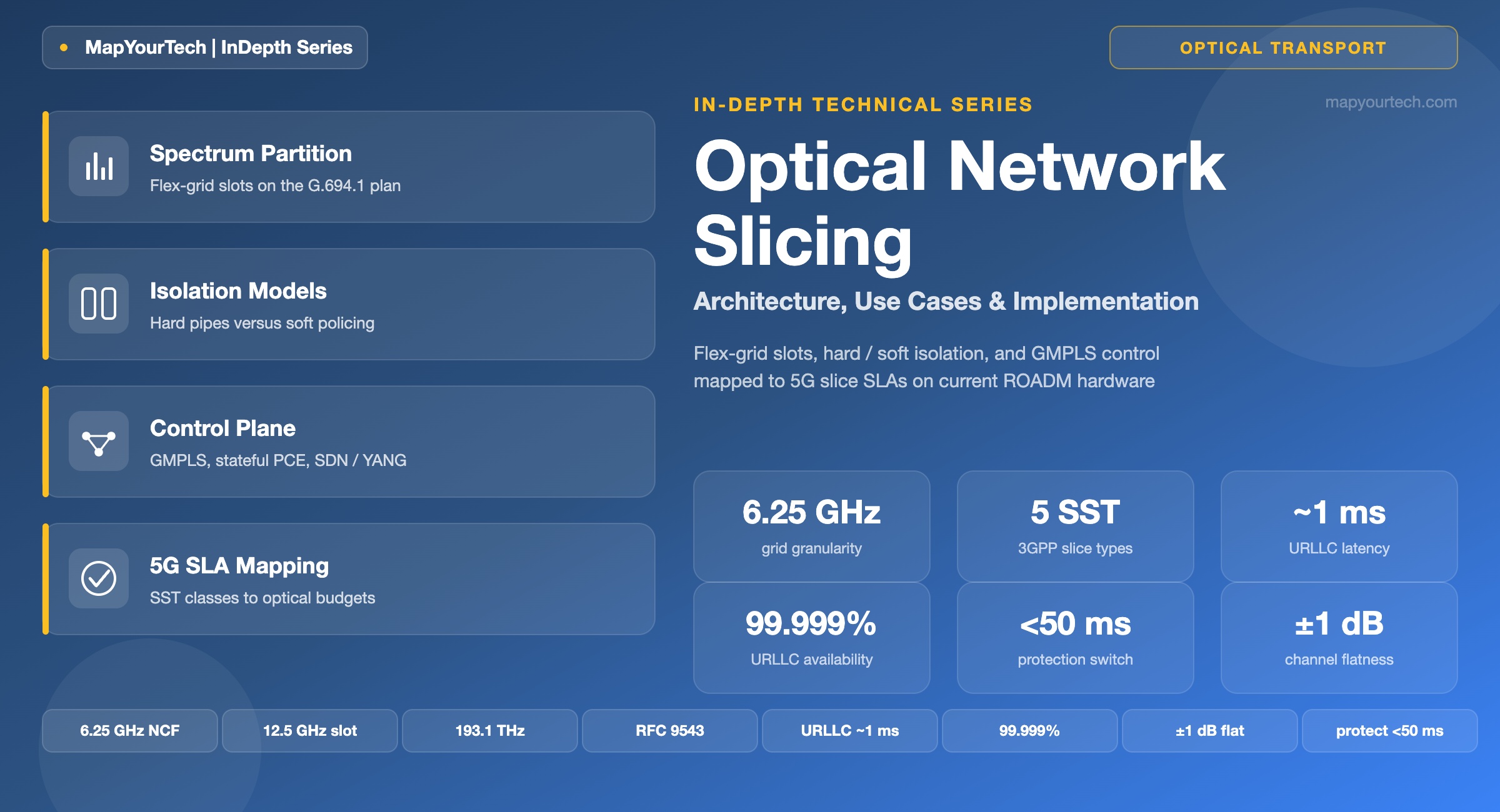
What an optical slice actually is, how flexible-grid spectrum is partitioned, where hard isolation ends and soft isolation begins, how the GMPLS and SDN control plane provisions a slice, how a 5G slice SLA lands on the optical layer, and how all of it runs on the flex-grid ROADM and OTN hardware in service today.
1. Introduction
A single fiber pair between two metro sites can carry a hyperscaler's data-center-interconnect traffic, a mobile operator's 5G backhaul, a bank's low-latency trading circuit, and a utility's control channel at the same time. Historically those tenants were separated by buying more fiber, more wavelengths, or more transponder shelves. Optical network slicing replaces that capital-heavy separation with a software construct: a set of network resources carved out of a shared optical substrate, bound to one customer or service, and held to explicit performance commitments. The slice looks and behaves like a private network to its tenant while riding the same amplifiers, wavelength-selective switches, and fibers as every other slice.
The term arrived in transport from the mobile world. The Internet Engineering Task Force gave it a formal frame in RFC 9543, A Framework for Network Slices in Networks Built from IETF Technologies (standard-specified, March 2024), which defines a network slice as connectivity between endpoints delivered with specific Service Level Objectives (SLOs) and Service Level Expectations (SLEs) over a common underlay. That definition is technology-agnostic on purpose. It is realized differently at each layer: as a VPN and queue policy in IP/MPLS, as a container in Optical Transport Network (OTN), and as a block of spectrum on a flexible-grid line system. This article is about the last two of those, the transport layers that a packet slice finally rides on, and about the seam where a 5G slice's latency and isolation promise becomes a real allocation of wavelengths, time slots, and switch ports.
Three things make optical slicing a 2026 topic rather than a research curiosity. The flexible grid standardized in ITU-T G.694.1 turned fixed 50 GHz lanes into arbitrary-width spectrum blocks that can be handed out per tenant. Coherent digital signal processing made each of those blocks independently measurable and tunable, so a slice's health can be observed without demultiplexing the whole comb. And the control plane matured: RFC 9543's Network Resource Partition, the CCAMP working group's OTN-slicing YANG model (a standards-track draft that expires in September 2026), and SDN controllers with path-computation engines now let an operator request a slice through a northbound interface and have it instantiated across the optical domain without touching a single patch panel. The rest of this deep dive works through the definition, the spectrum mechanics, the isolation taxonomy, the control plane, the 5G SLA mapping, the math, and the hardware, and ends where every honest slicing discussion ends: the trade-off between how strongly you isolate a slice and how much of the fiber you waste doing it.
2. What an Optical Slice Actually Is
Start with the object, not the abstraction. An optical slice is a bounded set of physical-layer resources reserved for a tenant: some spectrum, on some set of fibers, through some sequence of ROADM degrees, carried in some set of OTN containers, with a control-plane identity that ties them together and a performance contract attached. Strip away any one of those and it stops being a slice and becomes something weaker, a wavelength service, a leased lambda, a best-effort VPN.
RFC 9543 gives the abstraction a clean vocabulary that transport engineers should adopt because it removes ambiguity across layers. The customer buys an IETF Network Slice Service, expressed as connectivity between Service Demarcation Points (SDPs) with SLOs and SLEs. The provider realizes it inside the network as an IETF Network Slice, and the pool of underlay resources allocated to carry that slice's traffic is the Network Resource Partition (NRP). The NRP is the concept that maps most directly onto optics: it is the spectrum, the time slots, the buffer share, the wavelengths that belong to this slice and no other. A slice can be sliced again, hierarchically, and slices from different domains can be stitched end to end, which is exactly what a 5G end-to-end slice does when it crosses the Radio Access Network, the Transport Network, and the Core Network.
2.1 The three planes a slice touches
An optical slice is defined simultaneously in three planes, and confusion usually comes from collapsing them. In the data plane, the slice is the actual signal energy: a frequency slot on the fiber, or an ODU container in a time-division multiplex, carrying the tenant's bits. In the control plane, the slice is a set of forwarding and switching states with a slice identifier, computed and installed by GMPLS signaling or an SDN controller. In the management plane, the slice is a lifecycle object with a service model, an SLA, telemetry streams, and a northbound handle the tenant or an orchestrator can call. A well-built slice keeps these three consistent: the identifier in the control plane maps to the spectrum in the data plane and to the SLA object in the management plane, so a fault on one is observable on the others.
2.2 Why the optical layer is where isolation gets real
Packet-layer slicing can promise isolation, but it delivers it statistically, through queues, policers, and resource-partition markings that hold only as long as the scheduler behaves and the links are not oversubscribed past their design point. The optical layer can offer something packet layers cannot: a slice whose resources are physically disjoint from every other slice's, where one tenant's congestion, misconfiguration, or attack has no path to another tenant's signal. That is the property enterprises pay for and regulators sometimes mandate, and it is why the transport layers sit at the bottom of every serious end-to-end slice. For the packet side of the same story, the walkthrough on IP over DWDM architecture shows how a coherent router hands its wavelength to the very line system that a slice partitions.
2.3 From wavelength services to slices
The slice did not appear from nothing; it is the endpoint of two decades of the optical layer becoming programmable. Early DWDM sold a wavelength as a static circuit — a fixed lane at 50 or 100 GHz, planned by hand, provisioned by a truck roll. The wavelength-selective switch turned that lane into something a controller could route dynamically, and colorless-directionless-contentionless add/drop removed the physical port constraints that had tied a wavelength to a place. The flexible grid then removed the lane itself, and coherent DSP made each carrier independently tunable and measurable. Each step made the optical layer look less like a patch panel and more like a pool of allocatable resource. A slice is what you get when you add two things to that pool: a control-plane identity that names a subset of the resource, and an SLA that says what that subset must deliver. The mobile industry supplied the demand and the vocabulary; the optical industry already had the substrate. That is why slicing arrived as an integration problem — connecting a 5G orchestrator's slice request to a flex-grid line system's spectrum map — rather than as a new hardware category.
Takeaway: An optical slice is not a marketing overlay on a wavelength service. It is a named partition of real physical resources — spectrum, time slots, switch ports, fibers — bound to an SLA and kept consistent across the data, control, and management planes. The strength of the slice is the strength of that binding.
3. Spectrum Partitioning on the Flexible Grid
The physical substrate for spectrum-based slicing is the flexible grid defined in ITU-T G.694.1. The fixed grid it replaced allowed channel spacings of 12.5, 25, 50, and 100 GHz, all anchored at 193.1 THz (standard-specified). A 100G channel in a 50 GHz lane wasted spectrum; an 800G super-channel would not fit in one at all. The flexible grid removes the lane and replaces it with a frequency slot defined by two numbers: a nominal central frequency and a slot width. The central-frequency granularity is 6.25 GHz and the slot-width granularity is 12.5 GHz (standard-specified). Any allowed central frequency is f = 193.1 THz + n × 0.00625 THz, and any slot width is 12.5 × m GHz, where n is any integer and m is a positive integer.
Those two granularities are the reason the flexible grid works as a slicing substrate. The 6.25 GHz central-frequency step lets a slot with an odd multiple of 12.5 GHz sit directly against one with an even multiple, with no gap, so slices can be packed edge to edge. The 12.5 GHz slot-width step lets each fixed-grid spacing be reproduced exactly inside the flexible grid, so a slicing scheme can carry legacy fixed-grid channels and modern wide super-channels on the same fiber. The full treatment of these calculations, including the frequency-to-wavelength relationship, is in the reference on the G.694.1 DWDM channel grid, and the operational history of why the industry moved off the fixed grid is covered in the evolution to flexible-grid WDM.
3.1 Spectrum as a sliceable resource
Once spectrum is expressed as slots rather than lanes, it becomes a resource an operator can allocate the way a hypervisor allocates memory. A slice can be handed a contiguous frequency slot, say 193.1 THz to 193.5 THz across a chosen path, and told it owns that block exclusively. Inside its block the tenant may run whatever baud rate and modulation format its transponders support, because the line system is agnostic to what fills the slot as long as the tenant stays inside it and inside its power mask. This is the mechanism behind spectrum-as-a-service and behind alien-wavelength provisioning, where a third party's transponder lights a slice's spectrum through a provider's open line system. The multi-vendor mechanics of that arrangement are the subject of open line systems and multi-vendor coherent wavelengths.
3.2 Guard bands: the tax on spectral slicing
Slices carved in spectrum are not free at their edges. A frequency slot must include a guard band so that filter roll-off in cascaded wavelength-selective switches, laser frequency drift, and inter-slice crosstalk do not corrupt the neighbors. Early fixed-grid systems wasted enormous margin — a large fraction of a 100 GHz lane could be guard band. Modern coherent systems with digital pulse shaping and high-resolution wavelength-selective switches have pushed usable occupancy to within a few percent of the Nyquist limit, but the guard band never reaches zero, and every ROADM a slice traverses tightens the filter and widens the guard band it needs. The design of that margin is a discipline in itself, treated in depth in guard-band optimization. For slicing the consequence is direct: finer isolation between spectral slices costs spectrum, and that cost is the first term in the isolation-efficiency trade-off this article returns to.
3.3 Spectrum continuity and contiguity: the constraint that shapes every slice
A spectral slice is not just a slot on one link; it is the same slot on every link along its path. Two constraints follow from that, and they govern how a slicing control plane routes. Spectrum continuity requires that a slice occupy the same central frequency on all links it traverses, unless a wavelength converter is inserted — and converters are rare and costly in transparent optical networks, so in practice the slot must be identical end to end. Spectrum contiguity requires that the slot be a single unbroken block wide enough for the slice's signal plus guard band, not a set of scattered fragments. Together they turn slice placement into a search for a frequency slot that is simultaneously free and aligned across the whole path, which is a harder problem than routing a packet flow and the reason a path-computation element, not a distributed node, is the right place to solve it. When many slices come and go, these two constraints are also what makes spectrum fragmentation bite: free capacity exists but not as a continuous, aligned slot, so a new slice is blocked. Placing slices of different widths against these two constraints on a real line system, without stranding capacity in gaps too small to reuse, is the daily work of a spectrum planner. Figure 2 shows both constraints deciding the fate of three candidate slices on one path.
Read the Full Analysis with Premium
The remaining 78% of this article — the design numbers, trade-offs and field guidance — is part of MapYourTech Premium, along with the full premium library, courses and professional tools.
Optical Communications & Network Automation Expert | Author of 3 Books for Optical Engineers | Founder, MapYourTech
Optical networking engineer with nearly two decades of experience across DWDM, OTN, coherent optics, submarine systems, and cloud infrastructure. Founder of MapYourTech. Read full bio →
Follow on LinkedInRelated Articles on MapYourTech
You May Also Like
-
Free
-
July 11, 2026
-
Free
-
July 11, 2026
-
Free
-
July 11, 2026


