
Protection Switching Between Hollow-Core and SMF Paths
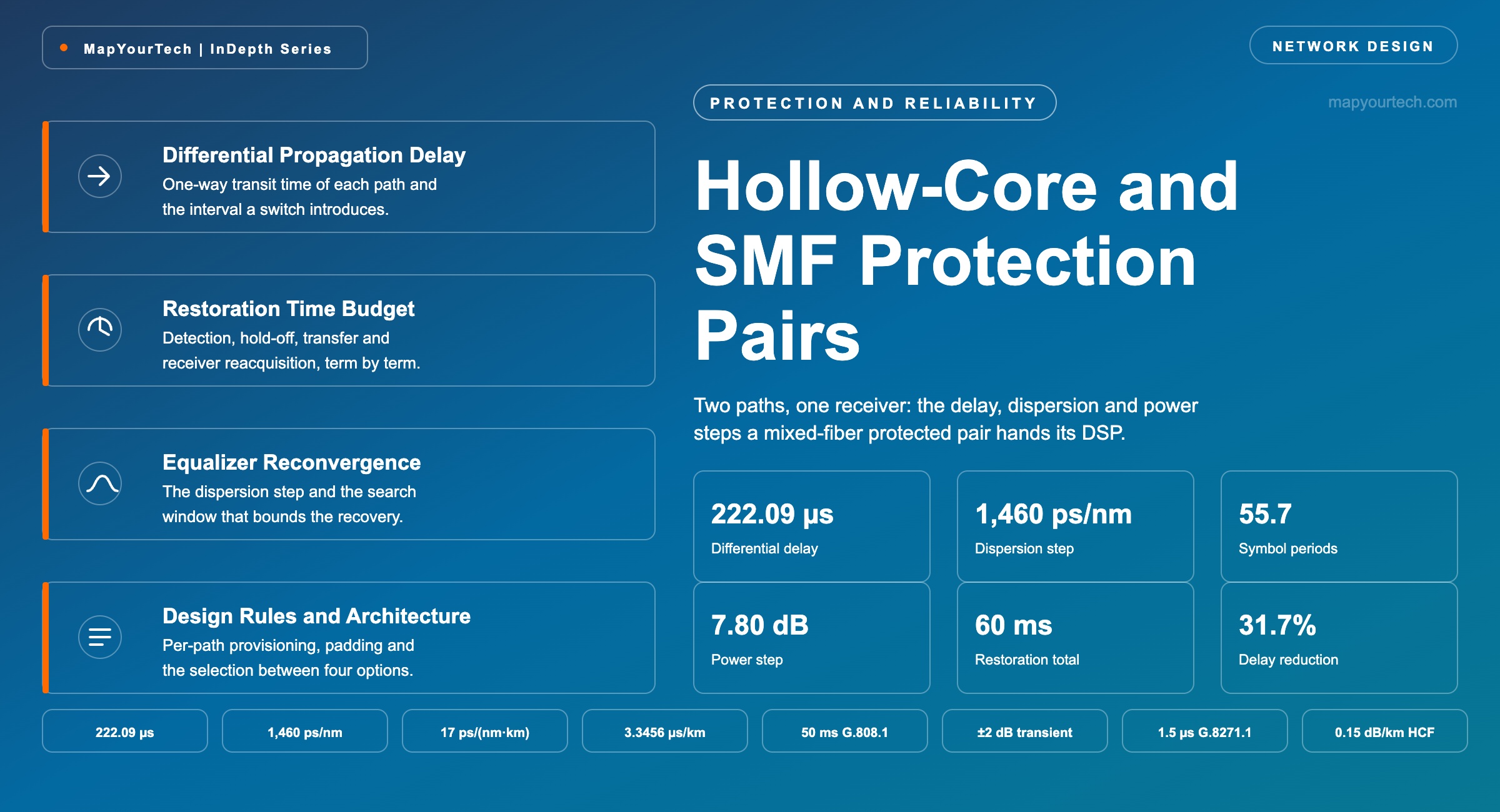
A working path in air and a protection path in glass differ by 222 µs of delay and 1,460 ps/nm of accumulated dispersion, and the receiver has to absorb both inside the switching budget.
A converged equalizer is a stored description of the path.
What You Will Learn
- Define differential propagation delay from group index and path length, and separate it from the differential group delay of Section 2.
- Compute the 222.09 µs one-way interval of the reference pair and separate it into a 97.95 µs length term and a 124.14 µs fiber-type term.
- Place the four terms of the restoration budget of Section 4 and show why a 222 µs delay interval consumes 0.4% of a 50 ms objective.
- Quantify the 1,460 ps/nm dispersion step of Table 4 as 55.7 symbol periods at 69 GBd, beyond the reach of a 20–30 tap adaptive equalizer.
- Build the per-path dispersion search window that converts a 10 s conformance bound into a 40 ms operational figure.
- Pad the 7.80 dB received power step of Section 7 to within the ±2 dB input transient tolerance the receiver rides through.
- Select unidirectional or bidirectional switching against the 1.5 µs time-error limit that a 111.05 µs path asymmetry violates.
- Construct the commissioning sequence of Section 9 and the observable set of Section 10 for a mixed-fiber protected pair.
1. Introduction
A 1+1 protected pair built with 80 km of anti-resonant hollow-core fiber (AR-HCF) on the working path and 100 km of G.652.D single-mode fiber (SMF) on the protection path delivers two signals that differ by 222.09 µs of one-way propagation delay and 1,460 ps/nm of accumulated chromatic dispersion (calculated from standard-specified group index and dispersion coefficients). Both signals originate at the same transmitter and terminate at the same coherent receiver. When the selector moves, the receiver does not see a brief interruption on one link; it sees the end of one link and the start of a different one, and every stored estimate it holds — dispersion, polarization rotation, timing phase, gain setting — describes the path that has just been removed.
Hyperscale deployment has made this a live configuration rather than a thought experiment. Microsoft has run HCF across multiple Azure regions since 2023 and contracted Corning and Heraeus in September 2025 to scale production, targeting deployment volumes in the tens of thousands of kilometres (vendor claim). AWS has begun production deployments across roughly ten data centres (vendor claim). Neither operator builds unprotected routes, and neither has enough HCF in the ground to build both halves of every protected pair from it. The mixed pair — one path in air, one in glass — is therefore the normal intermediate state of an HCF migration, not an edge case, and the same is true of any operator applying the selective-upgrade strategies that place HCF only on the links where it pays.
The engineering problem separates cleanly into two questions that are routinely merged. The first is whether the protection switch completes inside its objective, which is a question about detection, protocol exchange and selector operation, and which the fiber type changes by less than a millisecond. The second is what the receiver does after the selector has moved, which is entirely a question about how far apart the two paths are in dispersion, power, delay and polarization behaviour. A design that answers only the first question passes its switching-time test and then fails in service, because the protection event completes in 20 ms and the traffic returns 10 s later.
Scope covers single-carrier coherent line interfaces on a dedicated protected pair where one path uses AR-HCF and the other uses G.652.D SMF, at the optical layer and the Optical Transport Network (OTN) layer. It excludes photonic-bandgap hollow-core fiber, multi-core fiber, and mesh restoration onto a new wavelength, which inherits a different timing case altogether. The reference pair defined in Section 2 threads every section, so each number can be traced back to one configuration. The fiber physics behind the hollow-core side is developed in the hollow-core fiber fundamentals guide, and the protection mechanisms themselves in the optical network protection architecture reference.
Takeaway: A mixed-fiber protected pair passes two independent tests. The switch completes inside its objective almost regardless of fiber type; the receiver reacquires inside the objective only when the two paths have been characterised separately and provisioned separately.
2. Differential Propagation Delay Definition and Component Terms
Differential propagation delay is the difference between the one-way transit times of two parallel paths connecting the same pair of endpoints, measured in microseconds for metro and regional spans. Each path contributes its own transit time, set by its physical length and by the group index of the medium along it. The quantity is a property of the path pair, not of either path alone, and it persists for as long as both paths exist.
2.1 Distinctions From Adjacent Quantities
Four quantities sit next to differential propagation delay and get conflated with it, and each conflation produces a different design error.
Differential group delay (DGD) is the delay between the two principal states of polarization of a single signal on a single path, measured in picoseconds and produced by polarization mode dispersion. Differential propagation delay is the interval between two separate paths, measured in microseconds, and the two differ by six orders of magnitude on the reference pair — 1.00 ps against 222.09 µs.
Read the Full Analysis with Premium
The remaining 88% of this article — the design numbers, trade-offs and field guidance — is part of MapYourTech Premium, along with the full premium library, courses and professional tools.
You May Also Like
-
Premium
-
August 27, 2026
-
Premium
-
August 27, 2026
-
Premium
-
August 27, 2026