MapYourTech · MapYourBasics Series

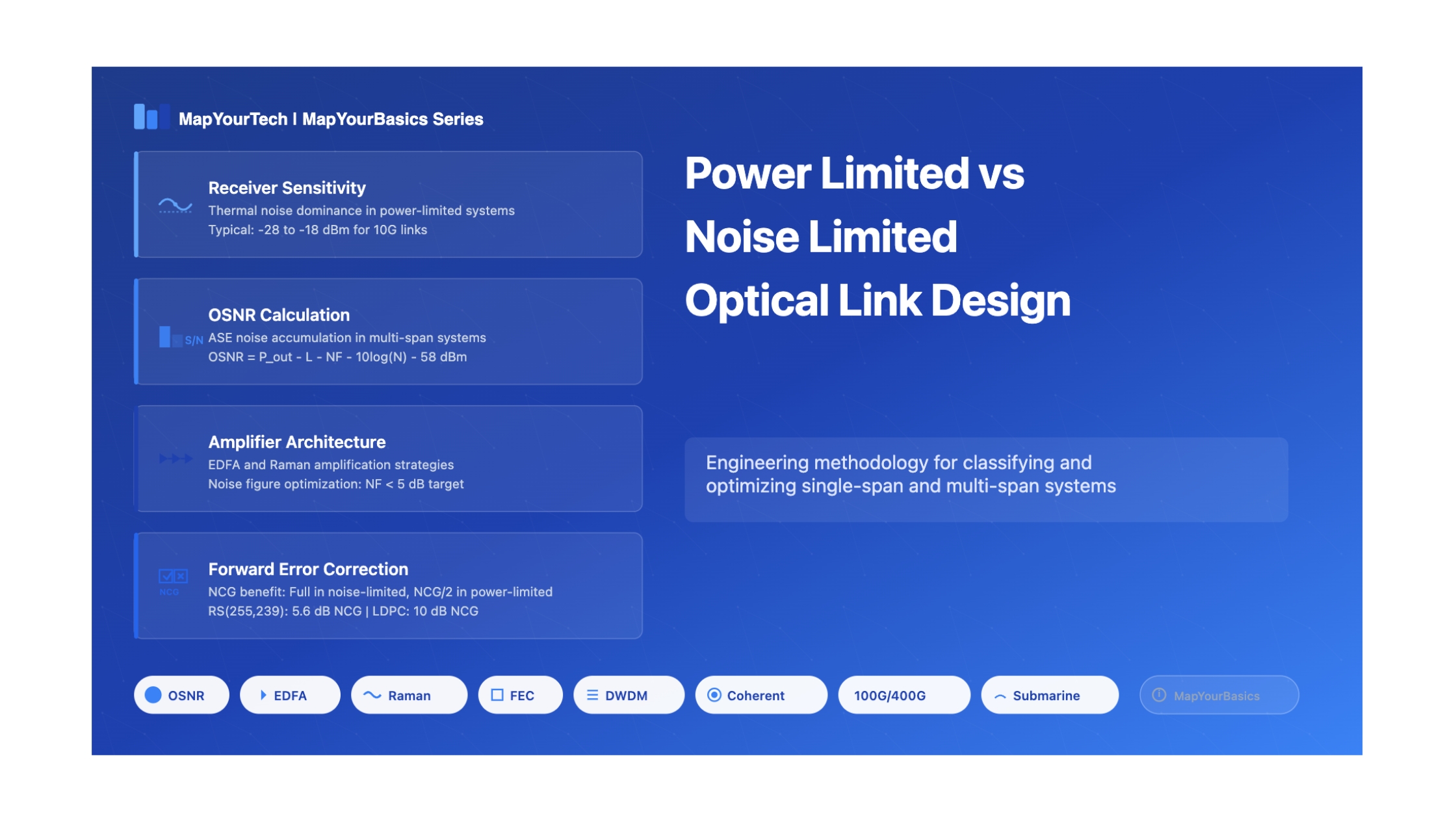
Power-Limited vs Noise-Limited Optical Link Design

Two regimes, two metrics, two scaling laws — whether a link is starved of signal or drowning in amplifier noise decides every component you buy.

Introduction

An optical link fails to close for one of two reasons, and they call for opposite fixes. Either too little signal power reaches the receiver to beat its electrical thermal noise — a power-limited link — or enough power arrives but it is buried under amplified spontaneous emission accumulated across a chain of optical amplifiers — a noise-limited link. The first is governed by receiver sensitivity in dBm and a power budget; the second by optical signal-to-noise ratio in dB. Confuse the two and the budget is wrong from the first line. This guide separates the regimes, gives the math for each, classifies the architectures that fall into them, shows where the boundary sits, and provides four calculators to run both kinds of budget.

The distinction in one line: a pre-amplifier in front of the receiver lifts the signal far enough above thermal noise that OSNR becomes the limit — it converts a power-limited link into a noise-limited one. The launch power of the source is what sets which regime you start in.

1. Fundamentals and Core Concepts

Power-limited links: the dominant noise is the receiver's electrical thermal noise, and performance is set by how much optical power survives to the receiver. This is the single-span case without optical amplifiers, where fiber attenuation pulls the signal below the level needed to beat thermal noise.

Noise-limited links: the dominant noise is ASE from the optical amplifiers, and performance is set by accumulated optical noise rather than raw signal level. This is the multi-span case with cascaded amplifiers, where ASE builds up and OSNR degrades from transmitter to receiver.

Physical origins

Receiver thermal noise comes from random electron motion in the load resistor and front-end amplifier. It is independent of received optical power and stays constant whatever the link looks like; without a pre-amplifier it exceeds shot noise and dominates. ASE noise comes from spontaneous emission in the amplifier gain medium being amplified along with the signal; in a multi-span chain each amplifier adds ASE that accumulates, and signal-spontaneous beat noise at the receiver overtakes thermal noise by a wide margin. The pivot is the pre-amplifier: place one before the receiver and it lifts the signal enough that thermal noise stops mattering, moving the system into the OSNR-governed regime.

Where the regime decides the design

Table 1: Limiting regime by link architecture
Scenario	Limiting factor	Typical applications
Single span, no amplifiers	Power-limited (thermal noise)	Metro, access, short-reach DCI
Single span with pre-amplifier	Noise-limited (ASE)	Long single-span terrestrial or festoon
Multi-span systems	Noise-limited (accumulated ASE)	Long-haul DWDM, submarine, metro-core
FEC-enhanced systems	Depends on architecture	Extended reach or relaxed power

Why the classification matters

The two regimes need different metrics, different components, and different scaling. Power-limited systems are specified by receiver sensitivity (minimum dBm) and reward premium transmitters and receivers; noise-limited systems are specified by required OSNR and reward low-noise-figure amplifiers and careful gain distribution. Distance scales differently too: in a power-limited link, doubling distance roughly doubles the loss to overcome (more transmit power or better sensitivity); in a noise-limited link, doubling distance doubles the amplifier count and costs about 3 dB of OSNR.

Takeaway: Decide the regime before the budget. Sensitivity in dBm answers a power-limited link; OSNR in dB answers a noise-limited one. The pre-amplifier is the switch between them, and launch power sets where you begin.

2. Mathematical Framework

Power-limited equations

SNR, thermal-noise limited

SNR = R_d²P_in² / (2q(R_dP_in+I_d)Δf + 4k_BTF_nΔf/R_L)

Where: R_d responsivity (A/W), P_in received power (W), q electron charge (1.602×10^-19 C), I_d dark current, Δf receiver bandwidth, k_B Boltzmann constant (1.38×10^-23 J/K), T temperature (K), F_n amplifier noise figure, R_L load resistance.

Receiver sensitivity (thermal-dominated)

P_rec = (Q / R_d) · √(4k_BTF_nΔf / R_L)

Where: Q ≈ 6 for BER 10^-9, Q ≈ 7 for BER 10^-12; typical P_rec is −28 to −18 dBm for 10G systems.

Power budget: P_TX − total loss ≥ P_rec + margin. Total loss is fiber attenuation plus connector and splice loss; the margin (typically 3–6 dB) covers aging, repairs, and variation.

Noise-limited equations

Multi-span OSNR

OSNR (dB) = P_out − L − NF − 10·log₁₀(N) + 58

Where: P_out per-channel amplifier output (dBm), L span loss = line-amplifier gain (dB), NF noise figure (dB), N number of line amplifiers, and +58 is the magnitude of 10·log₁₀(h·ν·ν_r) at 1550 nm over a 12.5 GHz (0.1 nm) reference. Amplifier gain cancels because OSNR is a ratio.

Accumulated ASE power

P_ASE = 2n_sp(G − 1)hνB × N

Where: n_sp spontaneous-emission factor (1.5–2 for EDFAs), G linear gain, B optical bandwidth, N amplifier count. The Q-factor maps to a bit error rate: Q = 7 (about 17 dBQ) gives BER 10^-12, Q = 6 gives 10^-9.

Practical Example — power-limited 80 km single span.
Fiber 0.25 dB/km × 80 = 20 dB; connectors/splices 2 dB; total 22 dB. TX 0 dBm → received −22 dBm. Against a −28 dBm receiver the margin is 6 dB, above the 3 dB target — the link closes and is thermal-noise limited.

Practical Example — noise-limited 800 km, 10 spans.
9 line amplifiers, span loss 20 dB, P_out +3 dBm/ch, NF 5 dB.
OSNR = 3 − 20 − 5 − 10·log₁₀(9) + 58 = 3 − 20 − 5 − 9.5 + 58 = 26.5 dB.
Against a 15 dB requirement for 10G NRZ that is 11.5 dB of margin — ASE-limited, with room to spare.

FEC behaves differently in each regime: with a net coding gain of 5.6 dB, a power-limited link without a pre-amplifier recovers only about half (2.8 dB) because thermal noise is independent of signal power, while a noise-limited link recovers the full 5.6 dB of relaxed OSNR because ASE scales with the signal. See Reed-Solomon FEC and pre/post-FEC thresholds.

3. System Types and Classification

Table 2: Link classification framework
Type	Architecture	Limiting factor	Key metric	Applications
1A	Single span, no amplifiers	Receiver thermal noise	Sensitivity (dBm)	Metro access, DCI
1B	Single span, booster only	Receiver thermal noise	Sensitivity (dBm)	Extended metro, campus
2A	Single span, pre-amp only	ASE (single amplifier)	OSNR (dB)	Long single span
2B	Single span, booster + pre-amp	ASE (two amplifiers)	OSNR (dB)	Very long single span
3	Multi-span line amplifiers	Accumulated ASE	OSNR (dB)	Long-haul, ultra-long-haul
4	Hybrid Raman + EDFA	Optimised ASE	OSNR (dB)	Premium long-haul, submarine

Component characteristics

Power-limited (Types 1A, 1B)

Transmitters run 0 to +5 dBm with low RIN and stable wavelength; receivers want high sensitivity (−28 to −18 dBm at 10G), where an avalanche photodiode can add 6–8 dB in the thermal-limited regime. Passive loss is minimised: connectors below 0.3 dB, splices below 0.05 dB, mux/demux 3–5 dB.

Noise-limited (Types 2A–4)

Amplifiers need NF below 5 dB (EDFA) or below 3 dB effective (Raman), 15–25 dB gain, flat gain (±0.5 dB across C-band), and output saturation above +17 dBm for DWDM. Placement matters: booster after the transmitter, in-line every 60–100 km, pre-amplifier before the receiver, and hybrid Raman+EDFA where noise budget is tight. Transmitters can run a moderate −3 to +3 dBm; receivers need 10–15 dB OSNR tolerance for NRZ, more for higher-order coherent formats.

Hybrid Raman + EDFA

Distributed Raman gain through the span plus a discrete EDFA at the span end gives a 2–4 dB lower effective noise figure, 3–5 dB better OSNR, and 20–30% more reach, at the cost of 200–500 mW pump power per wavelength and pump-signal management (SBS, FWM). Reserved for submarine and ultra-long-haul routes.

Table 3: Specification summary by regime
Parameter	Power-limited	Noise-limited (EDFA)	Noise-limited (hybrid)
TX power	0 to +5 dBm	−3 to +3 dBm	−3 to +3 dBm
RX sensitivity	−28 to −18 dBm	n/a	n/a
Required OSNR	n/a	13–18 dB	10–15 dB
Amplifier NF	n/a	4.5–6 dB	2–4 dB eff.
Max span loss	28–33 dB	20–25 dB	25–30 dB
Typical reach	80–120 km	600–1200 km	1000–2000 km

4. Effects and Impacts

Distance scaling

Power-limited reach falls linearly with loss: max distance = (P_TX − P_RX − margin − other losses) / fiber attenuation, so a 30 dB budget at 0.25 dB/km reaches 120 km and +3 dBm buys roughly 12 km. Noise-limited OSNR falls logarithmically: it drops 3 dB each time the span count doubles, and a 1 dB lower amplifier NF lifts OSNR by 1 dB across the whole link.

Table 4: Impact factors by regime
Factor	Power-limited effect	Noise-limited effect
Fiber attenuation	Direct 1:1 on reach	Needs higher amplifier gain
Connector loss	Each 0.1 dB ≈ 0.4 km lost	Minor if gain compensates
Amplifier NF	No effect (no amps)	1 dB NF = 1 dB OSNR loss
Transmit power	1 dB ≈ 4 km gained	1 dB = 1 dB OSNR gained
RX sensitivity	1 dB ≈ 4 km gained	No effect (thermal negligible)
Span count	No effect within budget	Doubling = 3 dB OSNR loss
Nonlinear effects	Minor (low power)	2–5 dB penalty at high power

Operating bands

Table 5: Performance bands (10G NRZ reference)
Power-limited margin	Noise-limited OSNR	Level	Typical BER
≥ 6 dB	> 20 dB	Excellent	< 10^-15
3–6 dB	15–20 dB	Good	10^-12–10^-15
1–3 dB	13–15 dB	Marginal	10^-9–10^-12
< 1 dB	< 13 dB	Poor	> 10^-9

A standard penalty budget sums chromatic dispersion (2 dB), PMD (1.5 dB), PDL (1 dB), nonlinearity (1.5 dB), filter concatenation (1 dB), aging/temperature (2 dB), and maintenance (1.5 dB) — about 10.5 dB total, which both regimes must carry on top of the bare budget.

5. Interactive Calculators

Four calculators: a power-limited link budget, a noise-limited multi-span OSNR, a side-by-side reach comparison, and an FEC coding-gain reach model. The reach comparison shows the pivot directly — adding a pre-amplifier replaces the sensitivity floor with a 15 dB OSNR floor and buys distance.

6. Design Techniques and Solutions

Power-limited optimisation

Transmitter power

High-power DFB or external modulation with a booster lifts the budget: +3 dBm buys about 12 km at 0.25 dB/km. Cost and consumption rise, and excess power risks nonlinearity. Best for 60–100 km metro.

Receiver sensitivity

An APD adds 6–8 dB in the thermal-limited regime; an optimised transimpedance front end cuts thermal noise; coherent detection adds 3–5 dB through balanced detection and DSP at the cost of complexity.

Loss minimisation

Fusion splices (0.05 dB) over mechanical (0.1–0.2 dB), low-loss connectors below 0.3 dB, thin-film filters over AWG, and modern low-loss fiber (0.18–0.20 vs 0.25 dB/km) together recover 2–4 dB — 8–16 km of reach.

Noise-limited optimisation

Amplifier noise figure

Two-stage EDFAs with 980 nm forward pumping, gain-flattening filters, and optimised erbium length target NF below 4.5 dB. A 1 dB NF cut is 1 dB OSNR across the link — roughly 20% more spans — at a 30–50% premium per amplifier.

Distributed Raman

Counter-propagating 1450–1480 nm pumps (100–300 mW each) give an effective NF of 2–4 dB and 3–5 dB OSNR, extending reach 30–50%. Watch SBS (broaden the pump), pump-pump spacing (>10 nm), and double-Rayleigh scattering.

Power loading

Raise per-channel power while OSNR-limited; back off once nonlinearity dominates. The optimum is where OSNR gain equals nonlinear penalty, typically −3 to +3 dBm/channel. Total output N×P_ch must stay within amplifier saturation — 80 channels at 0 dBm needs +19 dBm.

FEC coding gain

Table 6: FEC schemes and coding gain
FEC type	Net coding gain	Overhead	Applications
RS(255,239)	5.6 dB	6.7%	OTN standard, long-haul
BCH	3.8 dB	<1%	Low-overhead links
LDPC	8–10 dB	15–20%	Submarine, advanced coherent
Soft-decision FEC	10–11 dB	20–25%	Ultra-long-haul coherent

Takeaway: Apply the coding gain to the right metric. In a noise-limited link the full NCG relaxes the OSNR requirement; in a power-limited link without a pre-amplifier only half lands, because thermal noise does not move with the signal. The same modulation format can sit either side of the boundary depending on whether a pre-amp is present.

7. Design Methodology

The flow: define requirements, classify the regime, build the budget, allocate penalties, then verify margin. The classification gate is simple — no amplifiers and short reach means power-limited; any amplifier in the path means noise-limited.

START ├─ distance ≤ 80 km, margin ≥ 3 dB → no amplifiers (power-limited, Type 1A) ├─ distance ≤ 120 km → booster only (1B) or add pre-amp (noise-limited, 2A) ├─ distance ≤ 200 km → booster + pre-amp (noise-limited, 2B) └─ distance > 200 km → multi-span line amplifiers (noise-limited, Type 3)

Practical Example — 75 km metro, power-limited.
4×10G, BER 10^-12. TX 0 dBm; fiber 18.75 dB; passive 5 dB; total 23.75 dB → received −23.75 dBm. Against −28 dBm sensitivity the raw margin is 4.25 dB. Penalties (dispersion 1.5, PMD 0.5, aging 1.5) take 3.5 dB, leaving 0.75 dB — marginal. Adding BCH FEC (3.8 dB NCG) lifts the final margin to about 2.65 dB, or a +3 dBm transmitter takes it to 3.75 dB. Either closes it.

Practical Example — 960 km long-haul, noise-limited.
80×100G DP-QPSK over 12 spans (11 line amps), span loss 21 dB, premium EDFA NF 4.5 dB, +1 dBm/channel.
OSNR = 1 − 21 − 4.5 − 10·log₁₀(11) + 58 = 1 − 21 − 4.5 − 10.4 + 58 = 23.1 dB.
Penalties total 7 dB → net 16.1 dB; against a 13 dB QPSK requirement that is 3.1 dB of margin, and soft-decision FEC (11 dB NCG) drives post-FEC BER below 10^-15.

FEC SELECTION IF margin < 0 dB → infeasible without FEC deficit ≤ 6 dB → RS(255,239) deficit ≤ 10 dB → LDPC else → redesign architecture ELSE IF margin 0–3 dB → FEC recommended (RS or BCH) ELSE margin > 3 dB → FEC optional (future margin)

Common pitfalls: mixing sensitivity and OSNR metrics; forgetting the +58 bandwidth constant; under-allocating penalties; over-optimising for fresh fiber with no aging margin; setting amplifier gain that does not exactly match span loss, which breaks the OSNR accumulation.

8. Applications and Case Studies

Practical Example — metro ring optimisation.
Twelve offices, spans 15–95 km, all single-span power-limited. The 95 km span (fiber 23.75 dB + 6 dB passive = 29.75 dB) gave a −1.75 dB margin against a −28 dBm receiver — infeasible. Upgrading to +3 dBm transmitters and enabling FEC across all interfaces lifted the worst-span margin to about +4 dB, kept the fiber plant passive, and avoided roughly 36k in pre-amplifier cost. Power-limited links reward the combined transmitter-power-plus-FEC move before reaching for amplifiers.

Practical Example — 1200 km long-haul 100G upgrade.
Reusing 15 spans of 80 km with NF 5.5 dB EDFAs gave OSNR = 1 − 21 − 5.5 − 10·log₁₀(14) + 58 = 21.0 dB; after 7 dB of penalties the net 14.0 dB left only 1 dB over the QPSK requirement. Rather than replace 14 amplifiers, dropping per-channel power from +1 to −1 dBm cut nonlinearity (net penalty fell about 1 dB) and soft-decision FEC (11 dB NCG) relaxed the OSNR requirement to about 8 dB — a 5 dB margin, 20× capacity, and zero amplifier swaps.

Practical Example — 8500 km submarine design.
170 spans of 50 km (169 line amplifiers), span loss 13 dB, hybrid Raman+EDFA at NF 3.0 dB effective, −1 dBm/channel, DP-QPSK with probabilistic shaping and 12 dB SD-FEC.
OSNR = −1 − 13 − 3.0 − 10·log₁₀(169) + 58 = −1 − 13 − 3.0 − 22.3 + 58 = 18.7 dB.
After 8.5 dB of submarine penalties the net 10.2 dB clears a 9 dB FEC-relaxed requirement by 1.2 dB — the margin a 25-year transoceanic system runs on. Shorter 50 km spans beat 80 km here despite the higher amplifier count, because fewer dB per span means less ASE per hop.

Troubleshooting

Table 7: Symptom-to-cause guide
Symptom	Likely cause	Fix
High BER, power-limited	Insufficient received power	Raise TX power, improve sensitivity, cut loss
High BER, noise-limited	Low OSNR	Lower amplifier NF, raise channel power, add FEC
Margin fine but high BER	Dispersion or PMD	Add compensation or move to coherent
OSNR fine but high BER	Nonlinear effects	Reduce channel power, fix dispersion map
Drift over time	Aging, dirty connectors	Clean/replace connectors, repair fiber
FEC underdelivering	Pre-FEC BER above threshold	Improve raw OSNR or power first

Table 8: Quick-reference parameters
Parameter	Typical range	Best practice
Fiber attenuation (1550 nm)	0.18–0.25 dB/km	0.25 dB/km for conservative design
Connector loss	0.1–0.5 dB	Budget 0.3 dB each
Splice loss	0.01–0.1 dB	Fusion 0.05 dB
EDFA noise figure	4–6 dB	Premium < 4.5 dB
Raman effective NF	2–4 dB	Hybrid 3–3.5 dB
RX sensitivity (10G)	−18 to −30 dBm	−28 dBm typical
Required OSNR (DP-QPSK 100G)	10–13 dB	13 dB pre-FEC
Design margin	2–6 dB	3 dB minimum, 5 dB submarine

Main Points

1. Links are power-limited (receiver thermal noise) or noise-limited (amplifier ASE); the regime drives every design choice.

2. Use the right metric — sensitivity in dBm for power-limited, OSNR in dB for noise-limited. Never mix them.

3. A 1 dB lower amplifier NF lifts OSNR by 1 dB across the whole noise-limited link, making NF the decisive amplifier spec.

4. Noise-limited OSNR falls 3 dB each time the amplifier count doubles — the 10·log₁₀(N) reach limit.

5. FEC gives full NCG in noise-limited links but only half in power-limited links without a pre-amplifier.

6. A pre-amplifier flips a power-limited link into a noise-limited one by lifting the signal above thermal noise.

7. Carry 3–6 dB margin — more for submarine — for aging, temperature, and repairs over a 25-year life.

8. Hybrid Raman+EDFA lowers effective NF by 2–4 dB and is the lever for ultra-long-haul reach.

9. In noise-limited links there is an optimal channel power balancing OSNR gain against nonlinear penalty.

10. Test at worst case — longest wavelength, highest temperature, end-of-life margin.

References

ITU-T, Optical interfaces for multichannel systems with optical amplifiers (G.692), ITU-T Study Group 15.
ITU-T, Forward error correction for high bit-rate DWDM submarine systems (G.975.1), ITU-T Study Group 15.
ITU-T, Characteristics of a single-mode optical fibre and cable (G.652), ITU-T Study Group 15.

Sanjay Yadav, "Optical Network Communications: An Engineer's Perspective" — Bridge the Gap Between Theory and Practice in Optical Networking.

Developed by MapYourTech Team

For educational purposes in Optical Networking Communications Technologies

Note: This guide is based on industry standards, best practices, and real-world implementation experiences. Specific implementations may vary based on equipment vendors, network topology, and regulatory requirements. Always consult with qualified network engineers and follow vendor documentation for actual deployments.

Feedback Welcome: If you have any suggestions, corrections, or improvements to propose, please feel free to write to us at [email protected]