
Channel Width vs Baud Rate: The Interplay That Defines Coherent System Performance
How the relationship between spectral slot allocation and symbol rate drives every capacity, reach, and cost-per-bit decision in modern DWDM networks — from 50 GHz fixed-grid legacy to 300 GHz flex-grid 1.6T channels.
1. Introduction: Two Parameters, One System Trade-off
Every coherent DWDM channel occupies a defined slice of the optical spectrum. Two numbers govern what happens inside that slice: the baud rate — how many symbols per second the transmitter launches into the fiber — and the channel width — how many GHz the wavelength-selective switch (WSS) opens to let that signal pass. These two parameters are not independent. The baud rate determines the minimum spectral width the signal physically requires. The channel width determines the maximum spectral window the photonic layer will provide. The gap between them — or the lack of one — controls spectral efficiency, filter-induced penalty, inter-channel crosstalk, and ultimately the total capacity a fiber can carry.
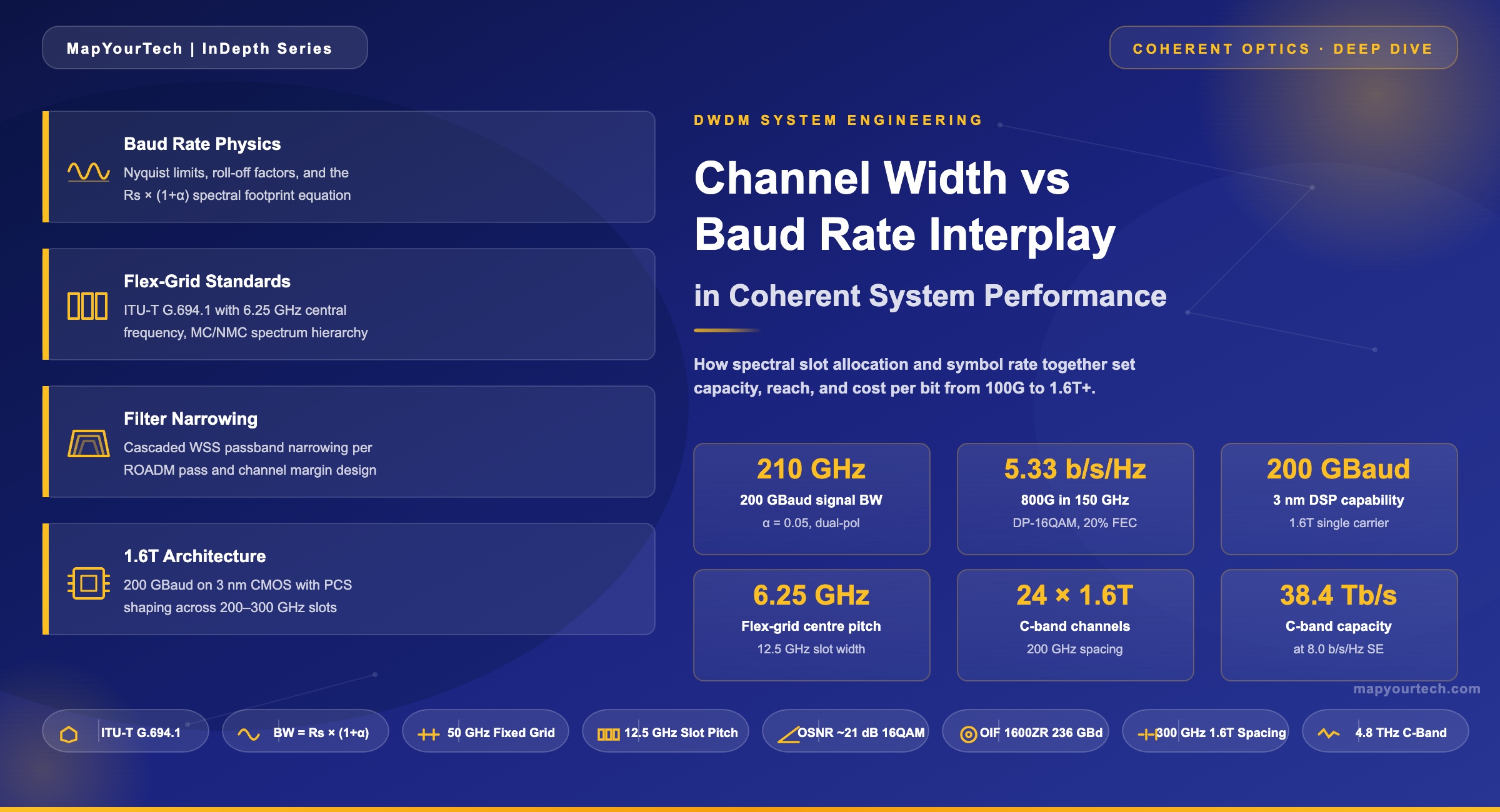
At 35 GBaud, a dual-polarisation QPSK signal carrying 100 Gb/s occupies approximately 37.5 GHz of spectrum with practical pulse shaping, fitting comfortably inside a 50 GHz fixed-grid slot with ~12.5 GHz of guard space on each side. At 95 GBaud, a shaped 400 Gb/s signal needs approximately 100 GHz of spectral occupancy and demands either a 112.5 GHz or 150 GHz flex-grid slot depending on the guard-band and filter-edge requirements. At 200 GBaud, a single-carrier 1.6 Tb/s signal requires approximately 200 GHz of channel width, and the entire C-band holds only 24 such channels. Each of these configurations represents a fundamentally different engineering trade-off between per-channel capacity, total fiber capacity, and transmission reach.
This article dissects that trade-off with quantitative precision. It covers the physics linking baud rate to occupied bandwidth, the standards framework that governs channel allocation, the impact of modulation format selection on the channel budget, the penalties imposed by cascaded optical filtering, and the practical design decisions operators face when planning networks from metro rings to transoceanic cables. The analysis draws on current-generation coherent platform capabilities, including systems operating at baud rates from 60 GBaud to 200 GBaud across both pluggable and embedded form factors.
Engineering context: The channel-width-to-baud-rate ratio is the single most underappreciated parameter in DWDM link engineering. An operator who packs 64 GBaud signals into 50 GHz channels will experience 3–5 dB of filter-induced penalty on the first ROADM pass. An operator who allocates 100 GHz to a 35 GBaud signal wastes 62.5 GHz of spectrum per channel — enough to carry an additional 100G wavelength. Both choices cost real money. Understanding the interplay prevents both.
2. Foundational Physics: Baud Rate, Spectral Width, and the Nyquist Limit
2.1 Baud Rate: The Clock of the Optical Channel
Baud rate (symbol rate, Rs) measures the number of discrete symbol transitions per second on the optical carrier. Each symbol carries log2(M) bits, where M is the modulation order — 2 for BPSK, 4 for QPSK, 16 for 16QAM, 64 for 64QAM. Dual-polarisation coherent detection doubles the information capacity by transmitting independent symbol streams on the X and Y polarisation states of the same wavelength. The gross data rate is therefore:
Rgross = Rs × log2(M) × Npol

Where:
  Rs     = Symbol rate (GBaud)
  M      = Modulation order (4 = QPSK, 16 = 16QAM, 64 = 64QAM)
  Npol  = Number of polarisations (2 for DP coherent)

Practical Example — 800G DP-16QAM:
  Rgross = 118 GBaud × 4 bits/sym × 2 pol = 944 Gb/s
  Net rate after ~15% SD-FEC overhead: ~800 Gb/s
The baud rate is the clock rate of the optical modulator and the analogue-to-digital converters inside the coherent DSP. Increasing it demands wider-bandwidth electro-optic components — modulators, drivers, trans-impedance amplifiers, and ADCs/DACs that can handle the analogue waveform without distortion. A 200 GBaud design requires approximately 100 GHz of electrical baseband bandwidth from the front-end optics and converters, compared to approximately 35 GHz for a 60 GBaud design. That 3× bandwidth increase is the primary reason why each baud-rate generation requires a new silicon process node and new photonic integration. For a deep exploration of how modulation format selection interacts with baud rate to determine bit rate, spectral width, and OSNR requirements, see the MapYourTech reference on Bit Rate vs Baud Rate in Optical Networks.
2.2 The Nyquist Limit and Occupied Bandwidth
The Nyquist-Shannon sampling theorem establishes that the minimum bandwidth required to transmit Rs symbols per second without inter-symbol interference (ISI) is Rs/2 Hz on each side of the carrier — a total one-sided bandwidth of Rs/2. In a dual-sideband system with no excess bandwidth, the minimum occupied bandwidth equals the baud rate itself: Bmin = Rs. This is the Nyquist limit, and it represents the theoretical minimum spectral footprint of a coherent signal.
Real transmitters cannot achieve this limit. Practical pulse-shaping filters introduce excess bandwidth characterised by the roll-off factor (α), which ranges from 0 (ideal rectangular spectrum, infinite time-domain sinc pulse) to 1 (fully excess bandwidth, smooth cosine pulse). The occupied bandwidth with a raised-cosine pulse shape is:
Read the Full Analysis with Premium
The remaining 89% of this article — the design numbers, trade-offs and field guidance — is part of MapYourTech Premium, along with the full premium library, courses and professional tools.