
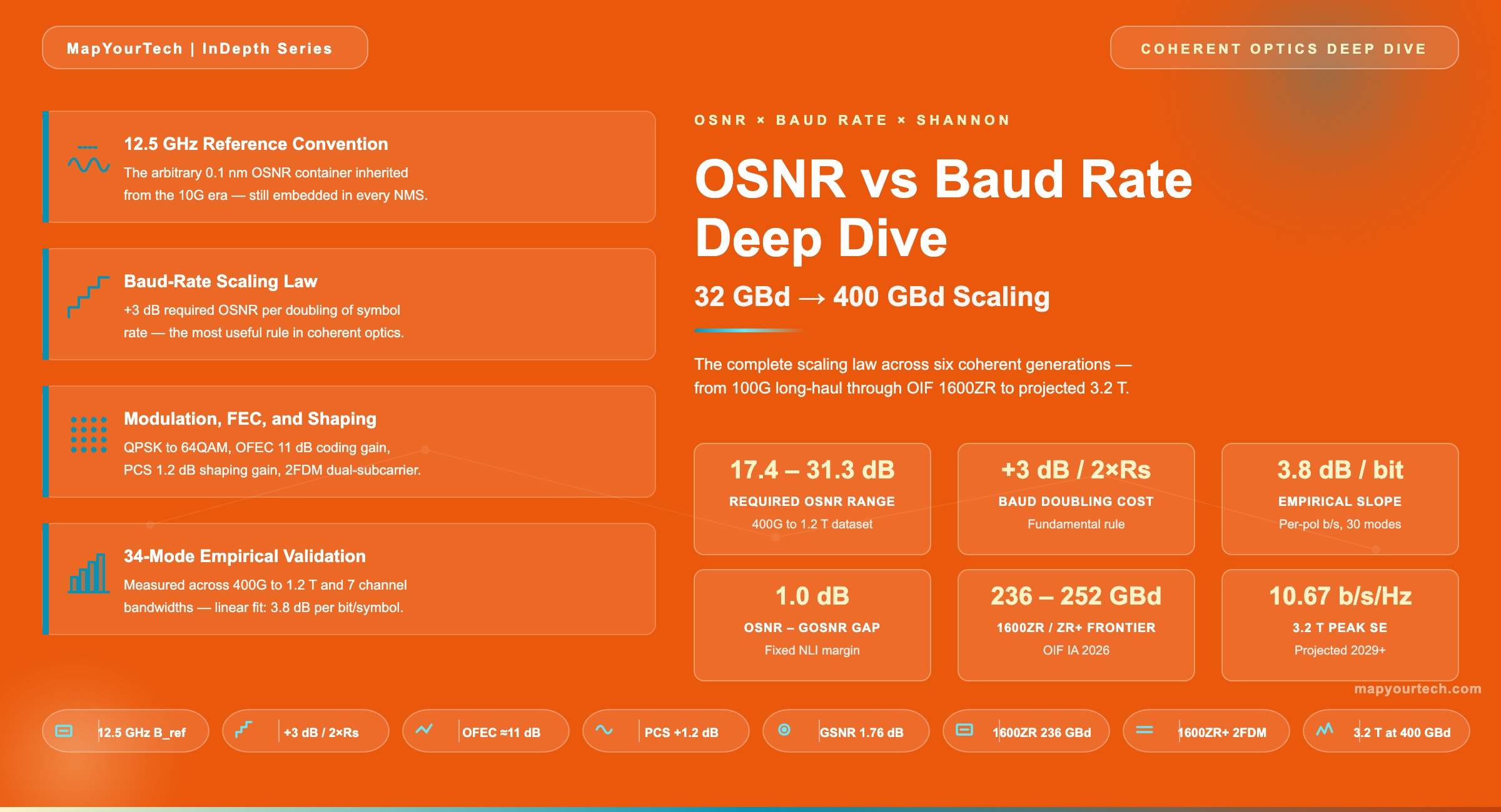
OSNR vs Baud Rate: The Coherent Transmission Deep Dive
Why the required OSNR at the receiver rises with every doubling of symbol rate, how the 12.5 GHz reference bandwidth hides the real SNR story, and what a 34-mode commercial modem dataset, extended with shipping 1.6 T platforms and the projected 2.4 T / 3.2 T roadmap, shows about the complete scaling law from 400G to 3.2 T.
Introduction
The required optical signal-to-noise ratio at the receiver of a coherent transponder rises by approximately 3 dB every time the symbol rate doubles — at fixed modulation order, fixed FEC, and fixed target bit-error rate. That single number governs how far a wavelength can travel, how many wavelengths fit on a fiber, and whether a 1.6 Tb/s pluggable can survive on an existing brownfield line system or needs a new one. Understanding why that 3 dB appears — and why the deployed numbers are often worse than 3 dB — is the difference between quoting a datasheet reach and engineering one.
The relationship between OSNR and baud rate is deceptively simple in its written form and genuinely subtle in its consequences. OSNR is a ratio measured over a fixed reference bandwidth. Baud rate is a signal parameter that sets the true noise-collecting bandwidth at the DSP input. The two bandwidths are not the same, and the scale factor between them is exactly where the 3 dB per doubling comes from. Once symbol rates climb above about 130 GBaud — which is now the mainstream for 800G coherent — the assumption that the 0.1 nm reference bandwidth is "narrower than the signal" breaks completely. At 236 GBaud for the OIF 1600ZR signal, the channel occupies roughly 19 times the reference bandwidth, and the headline OSNR number on the datasheet bears little resemblance to what the DSP sees.
This article works through the OSNR-to-baud-rate relationship in the depth the engineering decision deserves. It covers the reference-bandwidth convention from the ITU and IEC OSNR definitions, the per-modulation-format OSNR requirements from QPSK through 64QAM, the soft-decision FEC gain that shapes the deployed threshold, the implementation penalty that separates theory from silicon, the GSNR framework that replaces OSNR at high baud rates on nonlinear fiber, and the hardware constraints driving the 200 GBaud transition. A full section is dedicated to an empirical analysis of 34 published operating modes from a commercial coherent modem family spanning 400G through 1.2 T, extended with shipping 1.6 T platforms and projected 2.4 T and 3.2 T roadmap points — a vendor-agnostic dataset that validates the theoretical framework against real silicon across the full 400G-to-3.2 T coherent trajectory.
The OSNR Definition and Its Hidden Convention
OSNR is defined as the ratio of optical signal power to amplified spontaneous emission noise power, measured inside a specified reference optical bandwidth. In the overwhelming majority of industry practice the reference bandwidth is 0.1 nm at 1550 nm, which corresponds to 12.5 GHz of optical frequency. The convention predates coherent systems by more than a decade and was sensible when it was written — a 10 Gb/s NRZ signal with a 20 GHz spectral width comfortably encloses a 12.5 GHz noise slice, and an optical spectrum analyzer can interpolate the ASE noise floor between WDM channels.
The convention is now more historical than physical. IEC 61282-12 and CCSA YD/T 2147 generalize the definition to a user-specified reference bandwidth and to in-signal noise measurement through polarization nulling or spectral integration, but the 12.5 GHz number remains embedded in every datasheet, every network management system, and every planning tool. Engineers reading a spec sheet that says "required OSNR = 14.5 dB" are always reading that number in 0.1 nm reference bandwidth unless explicitly told otherwise.
The critical point is that the ASE noise is power spectral density — watts per hertz of optical bandwidth — and the 12.5 GHz slice is an arbitrary bookkeeping container. Double the symbol rate, and the signal spreads across a wider electrical bandwidth at the coherent receiver. The DSP sees noise integrated across that wider bandwidth, not across 12.5 GHz. The OSNR number stayed the same on the spectrum analyzer. The signal-to-noise ratio the DSP actually works with did not.
Two further subtleties shape every modern OSNR reading. First, the convention generally assumes noise is counted in a single polarization — but the optical spectrum analyzer measures both polarizations simultaneously and the signal in a dual-polarization coherent system spreads its power across both. The factor-of-two accounting appears differently in different textbooks and different planning tools, and mismatches are a frequent source of 3 dB discrepancies between models and field measurements. Second, in Nyquist-WDM deployments where channels are packed at spacing equal to or less than the symbol rate, there is no ASE-only gap between channels to interpolate, and the classical OSA method fails entirely. The integral method or in-service polarization nulling must be used instead, with accuracy boundaries that the optical performance monitoring toolchain must account for.
Takeaway: OSNR is a number quoted in a 12.5 GHz container — a container inherited from 10G systems and now roughly twenty times narrower than a modern 1.6 T signal. The container does not change when the signal widens. The actual SNR that drives the receiver bit-error rate does change, and the relationship between the quoted OSNR and the real SNR is governed entirely by the baud rate of the signal.
Baud Rate, Symbol Rate, and Occupied Bandwidth
Baud rate — symbol rate — is the number of independent modulation symbols transmitted per second. A 200 GBaud signal emits 2 × 10¹¹ symbols every second. Each symbol carries a constellation point, and the number of bits that constellation point encodes is the bits-per-symbol value, typically 2 for QPSK, 4 for 16QAM, 6 for 64QAM, with dual-polarization doubling those figures. Bit rate is the product of symbol rate and bits per symbol, pre-FEC. The distinction between baud rate, bit rate, and spectral width is worth having straight before reading the rest of this section — the three are often conflated in vendor datasheets, and the OSNR scaling argument depends on treating them as independent quantities.
The spectral footprint of a symbol stream is set by the Nyquist criterion and the pulse-shaping filter applied to suppress inter-symbol interference. An ideal Nyquist-shaped signal at symbol rate Rs occupies exactly Rs hertz of optical bandwidth. Real pulse-shaping filters use a raised-cosine or root-raised-cosine response with a roll-off factor α typically between 0.05 and 0.20 for modern coherent DSPs. The occupied bandwidth widens to Rs·(1 + α).
Three baud-rate eras mark the coherent generation boundary. The first generation of 100G coherent transceivers, deployed 2010–2014, operated at 28–32 GBaud and packaged one 100G wavelength into the classic 50 GHz ITU fixed grid. The second generation at 64 GBaud pushed 400G into 75 GHz flex-grid slots. The current mainstream — 130 to 140 GBaud — delivers 800G and 1.2 T per wavelength and requires 150 GHz flex-grid slots. The emerging 200 GBaud generation underpins 1.6 T and 2.4 T per wavelength and needs 200–300 GHz flex-grid slots. The ITU-T G.694.1 flex-grid framework is what made these jumps tractable — fixed 50 GHz grids became untenable at 64 GBaud and above.
One nuance often missed: the spec sheet baud rate is the symbol rate at the DSP output, not the filtered optical bandwidth. A 131.6 GBaud signal occupies approximately 138 GHz with a 5% roll-off, which fits inside a 150 GHz flex-grid slot with roughly 12 GHz of guard band. Push the same 131.6 GBaud into a 100 GHz slot that the ROADM filter narrows further, and the filter truncation introduces an OSNR penalty of 1–3 dB depending on the number of cascaded filters. That is the mechanism behind the spectral pre-emphasis knobs on many coherent transceivers — when an 8QAM signal at ≈42 GBaud passes through cascaded 50 GHz ROADM filters, transmit-side high-frequency boost counteracts the narrowing.
Read the Full Analysis with Premium
The remaining 88% of this article — the design numbers, trade-offs and field guidance — is part of MapYourTech Premium, along with the full premium library, courses and professional tools.
You May Also Like
-
Premium
-
September 2, 2026
-
Premium
-
September 1, 2026

-
Premium
-
September 1, 2026