Generic selectors
Exact matches only
Search in title
Search in content
Post Type Selectors
Articles
lp_course
lp_lesson
Back
HomeAnalysisFiber Physics and its Dynamics Optical Professionals Need to Know
Fiber-Physics-and-its-Dynamics-Optical-Professionals-Need-to-Know-MapYourTe...

Fiber Physics and its Dynamics Optical Professionals Need to Know

Last Updated: May 16, 2026
56 min read
51
Fiber Physics and its Dynamics Optical Professionals Need to Know
MapYourTech · InDepth Series · Fiber Fundamentals

Fiber Physics and its Dynamics Optical Professionals Need to Know

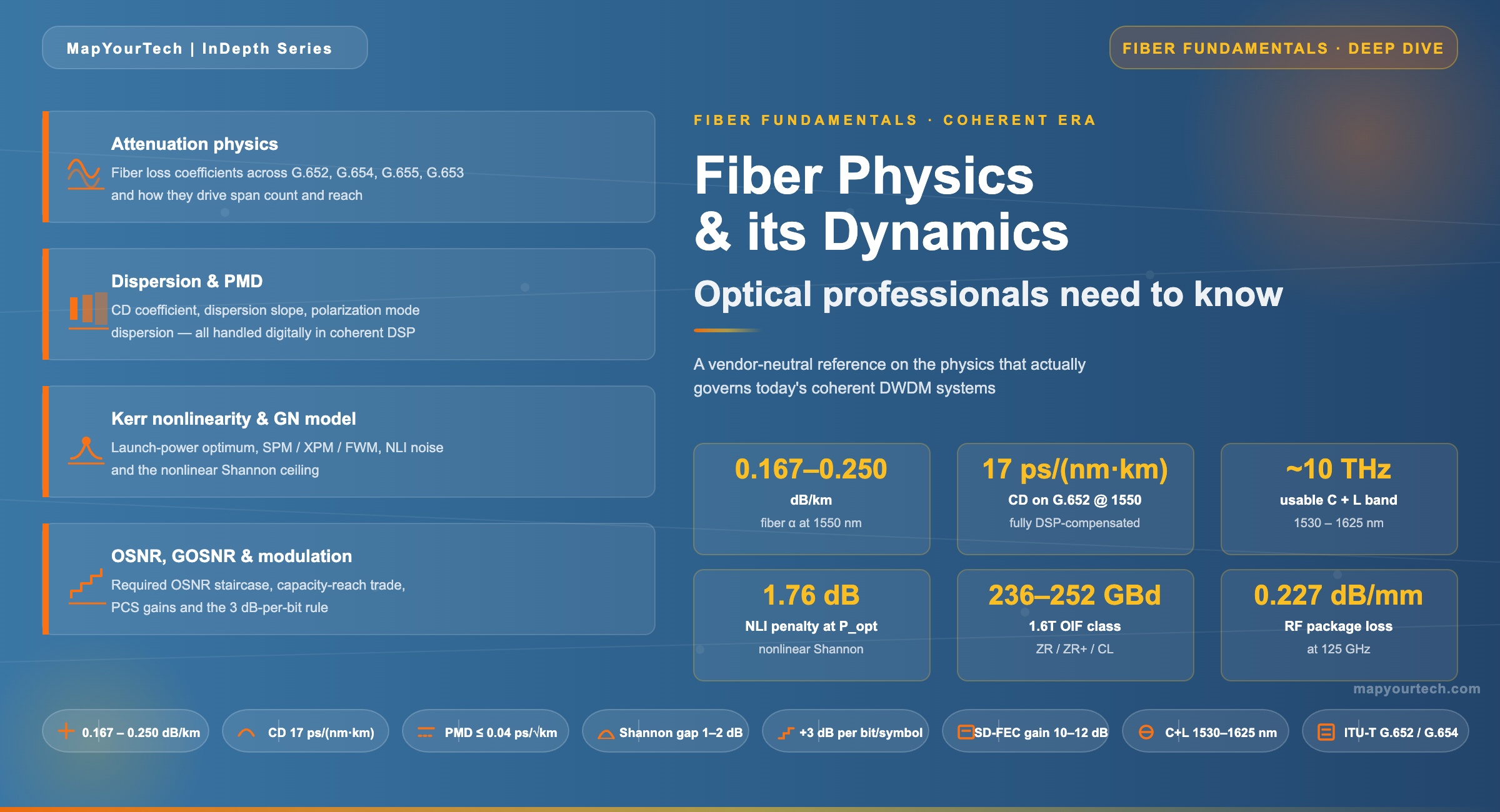
A working reference on the physics that actually shows up in a link budget, an alarm threshold, a modulation-choice decision, or a capacity forecast. Every claim here is grounded in the same ITU-T recommendations, fiber data sheets, coherent transceiver specifications, and deployed line-system parameters that practising engineers work with on a daily basis.

Attenuation · 0.167 – 0.250 dB/km CD · ~17 ps/(nm·km) at 1550 nm Baud rates · 35 → 252 GBaud OSNR · 0.1 nm reference BW C + L · ~10 THz usable Shannon gap · 1 – 2 dB

1. Introduction — why physics still governs

Every decision in an optical network — the reach of a wavelength, the modulation order a transponder selects, the margin a planner allocates, the alarm threshold a receiver trips — ultimately resolves to physics. The DSP can do extraordinary things with the complex optical field it receives. It cannot invent photons the fiber threw away, undo a polarization rotation that happened faster than its tracking bandwidth, or unwind a Kerr interaction that has already shifted phase between two channels. Fiber physics sets the ceiling. Every other engineering choice sits below it.

This article is an engineer's working view of that ceiling. It covers the phenomena that actually limit deployed coherent systems — attenuation, chromatic dispersion, PMD, Kerr-effect nonlinearity, ASE noise accumulation in amplifier chains — and the metrics (OSNR, GOSNR, required-OSNR-at-BER-threshold) that translate physics into engineering decisions. Where numbers appear, they are drawn from ITU-T fiber characterization data, vendor-published loss coefficients for deployed fiber types, and OIF-published symbol rates and channel widths for current-generation coherent interfaces.

The calibration target is: a newly-graduated optical engineer should finish this article with a complete mental model of how a link closes; a fifteen-year system architect should find at least one correlation or number that sharpens a planning assumption they have been using from memory. Every section is designed to answer three questions in sequence — what is the physical mechanism, what does it do in this system, and what happens if it is absent or fails.

How to read this article. Each impairment is introduced first by its physical origin, then by the quantitative scaling (the formula that an engineer carries in their head), and finally by the deployment consequence. The correlations section at the end connects the pieces — why lowering fiber attenuation shifts optimum launch power, why moving from C-band only to C+L changes the nonlinear interference spectrum, why higher baud rate intensifies RF package losses that had no practical impact at lower rates.

2. The spectrum — where light goes and why

Silica-based single-mode fiber is transparent enough to carry information across oceans, but only within a few specific wavelength windows. The boundaries of those windows are set by the same four physical mechanisms that determine which parts of the radio spectrum propagate through the atmosphere: intrinsic material loss, resonance absorption by impurities, Rayleigh scattering that scales as λ⁻⁴, and infrared absorption by silica itself at wavelengths above about 1600 nm. The result is a characteristic loss curve with a minimum near 1550 nm, a deep valley at 1310 nm, and a water-absorption peak near 1383 nm that modern fibers either suppress (low-water-peak variants) or exploit less aggressively (legacy fiber).

The ITU-T standardises the usable bands against this loss spectrum. The most-deployed fiber type today, ITU-T G.652.D standard single-mode fiber, is characterised for use from 1260 nm to 1625 nm, with the E-band water peak suppressed. G.654.E fiber — the ultra-low-loss, large-effective-area variant used on new submarine and long-haul terrestrial builds — targets 1530 – 1625 nm with attenuation as low as 0.15 – 0.17 dB/km and an effective area in excess of 110 µm². G.655 non-zero dispersion-shifted fiber was designed for the C-band era of dispersion-managed 10 Gb/s transport and is now a legacy constraint for coherent upgrades rather than a deployment target.

Fiber attenuation spectrum and deployed wavelength bands A plot of typical silica single-mode fiber attenuation from 1250 to 1650 nm showing the Rayleigh-dominated short-wavelength tail, the 1383 nm water peak, the 1310 nm second window, the 1550 nm C-band minimum, and the L-band extension to 1625 nm with infrared absorption onset beyond. 0.15 0.20 0.25 0.30 0.40 Attenuation (dB/km) 1260 1310 1383 1460 1530 1565 1625 1675 Wavelength (nm) O-band E + S band C-band L-band U-band minimum ~0.19 dB/km OH⁻ peak 1310 · zero-CD window
Figure 1 — Typical silica single-mode attenuation spectrum with ITU-T band labels. C-band plus L-band together occupy roughly 1530 – 1625 nm and provide the ~10 THz of low-attenuation, EDFA-amplifiable spectrum that underpins modern DWDM. Exact values are fiber-dependent; see Table 1.

The band names in Figure 1 are not marketing labels — they determine which amplifier technology is available. The C-band (1530 – 1565 nm) is the historical home of erbium-doped fiber amplifiers because the erbium energy levels produce efficient gain in exactly that window. The L-band (1565 – 1625 nm) also supports erbium gain but with a longer gain fiber and somewhat lower power efficiency. Together, C and L give approximately 10 THz of amplified spectrum — the substrate on which DWDM at scale is built. Everything outside those two bands is either shorter-reach IM-DD territory (1310 nm) or requires amplification technology other than EDFA, which is why the S-band and U-band have historically carried pump, supervisory, and maintenance traffic rather than revenue-bearing wavelengths.

A working engineer should internalise two spectrum facts. First, the total usable C+L spectrum is finite — roughly 9.6 THz under typical guard-band conditions, corresponding to about 96 channels at 100 GHz or 128 channels at 75 GHz spacing. Second, the attenuation differences between bands are real and directly enter span-loss calculations: a 1590 nm L-band wavelength on standard G.652 fiber sees approximately 0.02 dB/km more loss than a 1550 nm C-band wavelength, which over 80 km compounds to 1.6 dB of extra span loss — a margin an OSNR-limited design may not have.

Takeaway: Spectrum selection is a physics decision before it is a commercial decision. The attenuation curve sets the reachable bands; the amplifier technology sets which of those bands are economically viable; and the water peak and IR absorption tail fix the outer limits. Everything downstream — capacity, reach, channel plan — lives inside that envelope.

3. Attenuation — the first-order loss physics

Attenuation is the coefficient that converts kilometres of fiber into dB of signal loss. It is the first parameter an engineer plugs into a link budget, and it is the one most often taken from a nominal value rather than the actual characterisation of the deployed cable. The difference matters: a 0.02 dB/km error across an 80 km span is 1.6 dB — enough to push a margin-limited 16QAM channel below its required OSNR.

The physics has three contributors. Rayleigh scattering is the dominant mechanism below the infrared absorption tail; it arises from microscopic refractive-index fluctuations frozen into the glass during fiber draw and scales as λ⁻⁴. Material absorption — primarily from trace hydroxyl (OH⁻) ions — creates the 1383 nm water peak that makes E-band operation impractical on legacy fiber. Infrared absorption by the silica matrix itself becomes significant above 1600 nm and sets the long-wavelength cutoff. Waveguide imperfections (microbending, macrobending, splice losses) contribute additional loss that is not wavelength-selective but accumulates along the route.

Table 1 summarises the attenuation coefficients typically used for deployed fiber types. These values come from vendor-published reference tables and ITU-T fiber characterisation data. For link budget work, the key insight is the roughly 0.08 dB/km spread between the best G.654-class fiber and legacy dispersion-shifted fiber — a factor that over 1000 km of cable plant corresponds to 80 dB of total span loss difference, or approximately four additional amplifier spans' worth of ASE accumulation.

Table 1 — Attenuation coefficients at 1550 nm for common deployed fiber types
Fiber type ITU-T class Attenuation (dB/km) Effective area (µm²) Primary deployment
Ultra-low-loss large-Aeff (e.g. EX2000 class)G.654.E0.167~130New submarine and long-haul terrestrial
Ultra-low-loss, very large Aeff (e.g. EX3000 class)G.654.E0.168>150Latest-generation submarine
Pure silica core (PSC)G.654.B/C0.190~80 – 110Older submarine, low-loss terrestrial
Standard single-mode (NDSF)G.652.D0.200~80General terrestrial, metro, access
Low-water-peak NDSFG.652.D LWP0.200~80Metro with E-band utilisation
Large effective area (e.g. LEAF / ELEAF)G.6550.210~72Legacy C-band long-haul
AllWave (low-water-peak SMF)G.652.D0.210~80Early low-water-peak deployments
Metro-optimised NDSF variantG.6520.210~80Metro networks
Free-space pathn/a0.220n/aReference for free-space optical links
Dispersion-shifted fiberG.6530.250~50Legacy long-haul at 1550 nm (now unsuitable for C+L coherent)

The span-loss calculation that drops out of this table is straightforward in form but consequential in practice:

/* Total span loss for a single amplifier span */
L_span = α × D + L_splices + L_connectors + L_margin

where:
  α           fiber attenuation coefficient (dB/km)
  D           span length (km)
  L_splices   ~0.05 – 0.10 dB per fusion splice
  L_connectors ~0.20 – 0.50 dB per connector pair
  L_margin    fiber degradation reserve, 2 – 3 dB typical

Worked example — 80 km G.652.D span:
  L_span = 0.20 × 80 + 0.05×8 + 0.5×2 + 2.5
       = 16.0 + 0.4 + 1.0 + 2.5 = 19.9 dB

Same 80 km on G.654.E (α = 0.167):
  L_span = 0.167 × 80 + 3.9 = 17.3 dB
        2.6 dB improvement from fiber alone

That 2.6 dB is not a theoretical benefit. It is the gain an amplifier chain does not need to provide, which means an ASE contribution that is never added. Over an 8-span long-haul link, choosing G.654.E over G.652.D recovers about 2.6 dB of per-span OSNR budget — enough to change the modulation format that closes on a given route from 16QAM back to 32QAM, or to extend the reach of a 64QAM channel by roughly a factor of two. This is the cleanest, most linear trade in optical networking: pay more for better fiber, get more capacity out of the same route. The reason it is not universal is that the fiber is installed once and the cost is amortised over decades — upgrades target transponders, amplifiers, and DSPs instead.

3.1 Wavelength dependence and band tilt

Attenuation is not flat across C+L. A typical G.652.D fiber has about 0.19 dB/km at 1550 nm, rising to 0.21 – 0.22 dB/km at the L-band edge near 1620 nm. In a fully loaded C+L system with 96+ channels per band, this wavelength-dependent loss manifests as a tilt across the spectrum after each span. Amplifiers flatten it imperfectly — EDFA gain flatness is typically 1 – 2 dB peak-to-peak after a gain flattening filter — and stimulated Raman scattering (SRS) inside the fiber transfers power from shorter to longer wavelengths, adding another 1 – 3 dB of tilt across the full C+L window. Every line system deploys dynamic gain equalisers (DGEs) or wavelength-selective switches with DGE capability to keep the tilt inside the per-channel OSNR budget.

For design, the practical rule is that wavelengths near the band edges carry 1 – 2 dB less OSNR margin than band-centre wavelengths in a fully loaded system. Channel plans that put high-rate, margin-limited services on edge wavelengths are fighting physics. The more robust approach is to keep the hardest modulation formats in the middle of the band and accept that edge slots will carry lower-rate, higher-margin traffic.

Takeaway: The deployed fiber's attenuation coefficient is the single most leveraged physical parameter in the link budget. A 0.03 dB/km improvement is the difference between long-haul and regional reach on the same route. Every engineer should know the actual α of the fiber they plan on, not the textbook value for the generic ITU class. When a route has mixed fiber types, plan against the worst section — because the OSNR-limited channel will always be the one that transits the highest-loss segment.

Span count as a function of fiber attenuation at fixed route length Chart showing how the number of amplifier spans required for a 1000 km route varies with fiber attenuation coefficient. Higher-loss fibers force shorter individual spans to keep per-span loss below the receiver sensitivity limit, producing more ASE accumulation and lower OSNR at the destination. Span count for 1000 km route — with OSNR penalty vs. fiber type Amplifier spans needed 5 8 11 14 17 20 OSNR penalty vs. best fiber (dB) 0 1.5 3.0 4.5 6.0 G.654.E ULL 0.167 dB/km G.654.B/C PSC 0.190 dB/km G.652.D 0.200 dB/km G.655 LEAF 0.210 dB/km G.655 wideband 0.220 dB/km G.653 DSF 0.250 dB/km 9 10 11 11 12 13 +1.6 dB Span count OSNR penalty vs. best fiber (dB)
Figure 2b — For a fixed 1000 km route at a 22 dB per-span loss ceiling, fiber attenuation directly controls both span count and accumulated ASE. Moving from G.654.E (9 spans, reference OSNR) to G.653 (13 spans) costs ~1.6 dB of cumulative OSNR — enough to demote the achievable modulation format from 32QAM to 16QAM on the same route.
Attenuation coefficient comparison — ten deployed fiber types Horizontal bar chart comparing typical attenuation coefficient at 1550 nm across ten fiber types from ultra-low-loss G.654.E at 0.167 dB/km up to legacy G.653 dispersion-shifted fiber at 0.250 dB/km, showing the roughly 50 percent performance spread between best and worst fiber still installed in deployed plant. Fiber attenuation at 1550 nm — deployed fiber types 0.15 0.17 0.19 0.21 0.23 0.25 Attenuation coefficient (dB/km) G.654.E · ULL large-Aeff 0.167 dB/km G.654.E · ULL very-large-Aeff 0.168 G.654.B/C · pure silica core 0.190 G.652.D · standard SMF (NDSF) 0.200 · reference G.652.D · low water peak 0.200 G.655 · LEAF / ELEAF 0.210 G.652.D · AllWave 0.210 G.652 · metro-optimised 0.210 (free-space reference) 0.220 G.653 · dispersion-shifted 0.250 · legacy only ← lower loss · longer reach higher loss · shorter reach →
Figure 2a — Attenuation coefficient at 1550 nm for ten deployed fiber types. The gap between the best (G.654.E at 0.167 dB/km) and the worst still in service (G.653 at 0.250 dB/km) is 0.083 dB/km — a factor that, over 1,000 km of cable, changes total loss by 83 dB and effectively determines whether a route can run coherent DWDM at high spectral efficiency.
Premium Article — Free 22% Preview

Read the Full Analysis with Premium

The remaining 78% of this article — the design numbers, trade-offs and field guidance — is part of MapYourTech Premium, along with the full premium library, courses and professional tools.

Instant access · Cancel anytime · 48-hour trial available
Sanjay Yadav

Optical Communications & Network Automation Expert | Author of 3 Books for Optical Engineers | Founder, MapYourTech

Optical networking engineer with nearly two decades of experience across DWDM, OTN, coherent optics, submarine systems, and cloud infrastructure. Founder of MapYourTech.

Follow on LinkedIn

You May Also Like

15 min read 6 0 Like Connector Types and Their Loss Budgets: SC, LC, MPO Skip to main content MapYourTech...
  • Free
  • July 11, 2026
16 min read 6 0 Like Cooled vs Uncooled Lasers: The Pluggable Power Trade-off Skip to main content MapYourTech |...
  • Free
  • July 11, 2026
16 min read 7 0 Like Automation Blast Radius: Scoping What a Bad Intent Can Touch Skip to main content...
  • Free
  • July 11, 2026

Course Title

Course description and key highlights

Course Content

Course Details