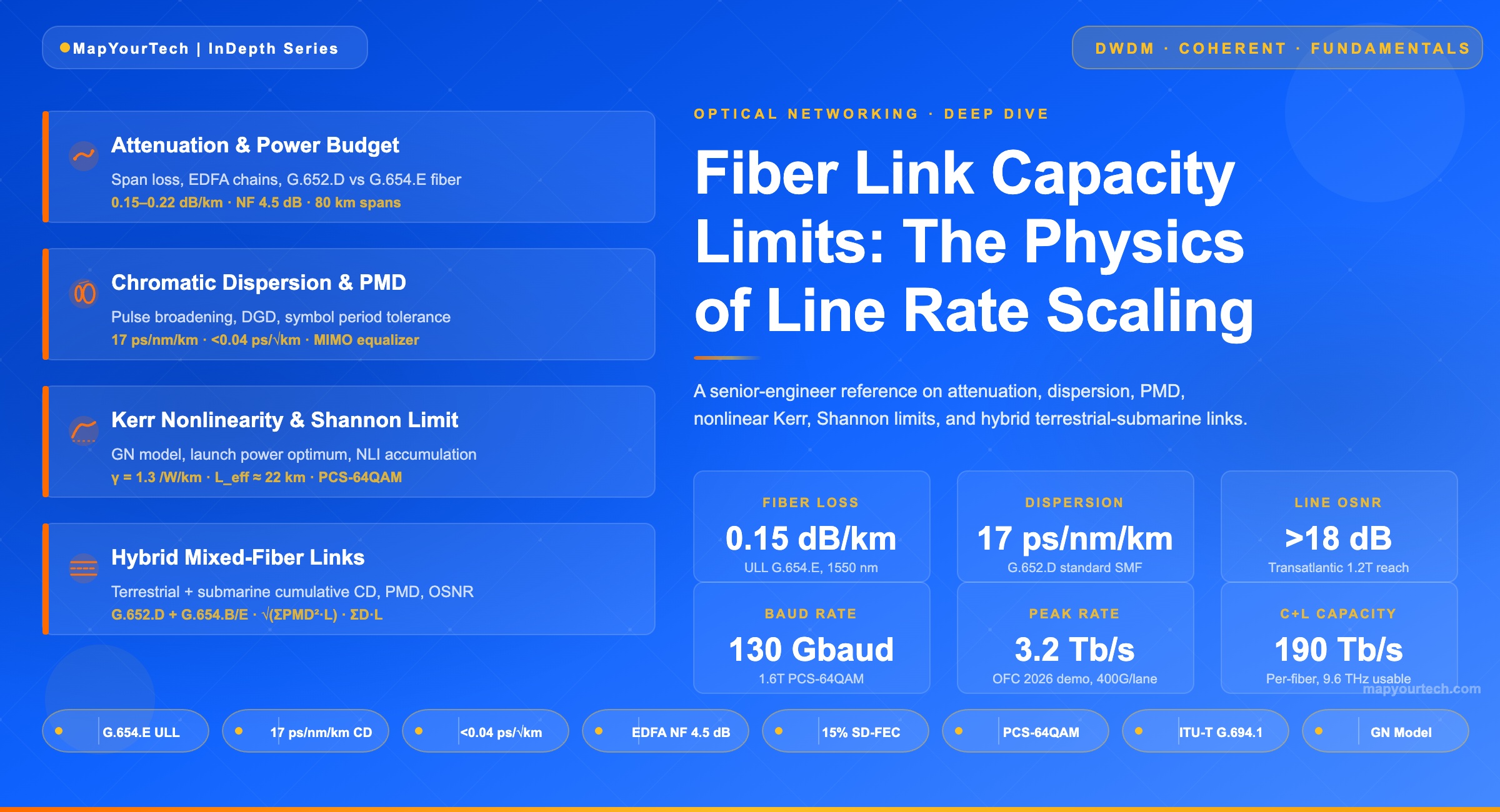
Fiber Link Capacity Limits: The Physics Behind Line Rate Scaling
Why a single wavelength on a glass strand cannot scale to arbitrary data rates. A complete tour of the physical barriers that govern how many bits per second a fiber channel can carry, from attenuation and dispersion to the nonlinear Shannon limit and the modern push toward 1.6 Tb/s and 3.2 Tb/s coherent transport.
1. Abstract and Executive Summary
The line rate of a single wavelength channel on optical fiber is not a free parameter that engineers can raise at will. It is the outcome of a layered physical negotiation between launch power, optical bandwidth, noise accumulation, dispersive pulse spreading, and the Kerr-induced nonlinear penalty that grows with every additional milliwatt of light pushed into the glass. Modern coherent transceivers have turned what was once a hard wall into a gentle curve — but a curve that still bends sharply downward past a well-defined operating point.
This article unpacks every physical mechanism that caps the data rate a fiber channel can carry. It starts with attenuation, the simplest loss, and moves through chromatic dispersion (CD) and polarization mode dispersion (PMD), the two dispersive impairments that consume pulse-width budget. It then treats the Kerr nonlinearity as the dominant ceiling for high-capacity coherent systems, where the Gaussian noise (GN) model, developed by Poggiolini and colleagues, provides a closed-form prediction of how nonlinear interference accumulates. Optical signal-to-noise ratio (OSNR) accumulation from cascaded erbium-doped fiber amplifiers (EDFAs) then sets the lower limit on receiver SNR for a given modulation format and forward error correction (FEC) scheme.
The second half of the article connects these physical limits to the engineering levers that have delivered four successive generations of coherent transceivers: 100G class-1 at 32 Gbaud on 50 GHz grids, 400G class-2 at 68 Gbaud on 75 GHz grids, 800G class-3 at 130 Gbaud on 150 GHz grids, and the emerging 1.6T class-4 at 240–272 Gbaud on 300 GHz grids. Each doubling of line rate has required a roughly doubled baud rate, a wider channel slot, and a more sensitive DSP that compensates CD electronically, tracks PMD adaptively, and extracts the most bits per dimension the channel will allow. At OFC 2026, vendors demonstrated 3.2T pluggables based on 400G-per-lane PAM4 for short-reach datacom and previewed 12.8T architectures for AI-scale infrastructure.
The central message is a conservation law. If a designer wants more bits per second through a fixed fiber, they can push three knobs: raise the baud rate (which buys bandwidth and worsens dispersion and noise tolerance), raise the spectral efficiency through denser modulation (which buys bits per symbol and worsens OSNR tolerance), or shorten the reach (which buys margin by reducing cumulative impairments). These three knobs trade against each other along a surface whose shape is set by the nonlinear Shannon limit. No amount of DSP or FEC ingenuity will move that surface; only a different fiber, a different amplifier, or additional spatial modes will.
Who should read this: optical system engineers sizing DWDM links, submarine cable designers preparing for next-generation repeaters, DCI architects evaluating 1.6T pluggable deployment, and research engineers exploring hollow-core fibers, multiband amplification, or space-division multiplexing. The depth assumes familiarity with basic fiber optics and coherent detection; every formula is derived in context.
2. Introduction and Context
Ask any optical engineer why a 100 Gb/s channel cannot simply be turned into a 1 Tb/s channel by scaling up the electronics, and the honest answer is a list rather than a number. The list reads like a textbook table of contents: attenuation sets how much power the receiver sees, dispersion sets how cleanly each symbol arrives, nonlinearity sets how much power can be launched without distorting neighboring channels, and noise sets how many bits per symbol the receiver can reliably decode. Each of these four forces scales differently with distance, with baud rate, and with modulation order. Their joint optimum is a narrow operating point, and that operating point defines the channel capacity for a given link.
The reason this matters today is economic, not academic. Global IP traffic has grown at roughly 25 to 30 percent per year for two decades. AI training clusters have pushed datacenter interconnect (DCI) bandwidth demands to hundreds of Tb/s per rack row. Hyperscale operators have deployed 400ZR in volume, are now deploying 800ZR, and are preparing 1.6T trials. Submarine cables commissioned in 2025 carried 24 to 40 Tb/s per fiber pair across transoceanic distances using 130 Gbaud probabilistically shaped 64QAM. Meanwhile the installed base of G.652 standard single-mode fiber (SMF), deployed in billions of kilometers over the last thirty-five years, has not changed its physical properties. The same glass that carried 2.5 Gb/s SDH in 1995 carries 800 Gb/s coherent wavelengths today. What changed is everything at the ends of the fiber, and how aggressively those ends can approach the physical limits of the middle.
Understanding where those physical limits come from is the subject of this article. The framing is engineering-oriented rather than purely physical: every mechanism is described with its practical consequence — how many dB of OSNR it consumes, how many picoseconds of pulse broadening it produces per kilometer, how many kilometers of reach it removes from a given modulation format. Where useful, we reference standard values from ITU-T G-series recommendations and typical coherent-transceiver performance envelopes as shipped by major vendors in 2025 and 2026.
2.1 What Do We Mean by Line Rate?
Line rate is the gross per-wavelength data rate measured at the client-facing interface before removing FEC and framing overhead. A 400 Gb/s coherent wavelength at 64 Gbaud PM-16QAM actually transmits about 470 Gb/s of raw symbols, of which roughly 15 percent is FEC overhead and a few percent is framing and training-sequence overhead. The useful payload rate the customer pays for is 400 Gb/s. When engineers discuss the scaling from 100G to 1.6T, they mean this payload rate.
The line rate splits into three factors: baud rate (how many symbols per second leave the modulator), bits per symbol (how much information each symbol encodes in amplitude, phase, and polarization), and FEC code rate (what fraction of the raw bits are payload after error correction). Increasing any of these factors increases the line rate, but each comes with a different physical penalty. Baud rate directly widens the optical spectrum the channel occupies and multiplies the required receiver bandwidth. Bits per symbol increase the minimum SNR the receiver needs to decode without errors. FEC code rate rises come from stronger codes that are more complex to implement and add latency.
2.2 The Three-Dimensional Scaling Surface
A useful mental model is to picture a three-dimensional surface whose axes are data rate, reach, and spectral efficiency. For any fiber type and amplifier chain, this surface has a maximum ridge defined by the nonlinear Shannon limit. Every real transceiver sits somewhere on or below this ridge. Modern coherent DSP has moved the operating point very close to the ridge for standard SMF in the C-band. Moving above the ridge means the channel cannot exist — the noise, nonlinearity, and dispersion conspire to make error-free decoding impossible regardless of how much margin the DSP adds.
Equivalently, every practical engineering decision — which modulation format to use, how many dB of launch power to apply per channel, how close to pack neighboring channels, how long a span to install between amplifiers — maps to a point on this surface. The rest of this article is about how each of the physical limits shapes the surface and where the current frontier sits.
3. Historical Evolution of Fiber Channel Capacity
The history of per-wavelength line rate is also the history of how each physical limit moved from being the binding constraint to being routinely compensated. Following that progression helps explain why specific limits matter at specific points in the technology curve, and why the current frontier looks so different from the one engineers faced twenty years ago.
3.1 First Generation: Direct Detection at 2.5 and 10 Gb/s
Early SDH and SONET systems in the 1990s ran at 2.5 Gb/s (STM-16, OC-48) and later 10 Gb/s (STM-64, OC-192) on a single wavelength using on-off keying with direct detection. The binding physical constraint was chromatic dispersion. At 10 Gb/s over standard G.652 SMF, accumulated CD beyond about 60 km caused eye closure severe enough to degrade BER below the error threshold. Operators compensated by inserting dispersion compensation modules (DCMs) built from dispersion-compensating fiber (DCF) with large negative dispersion coefficient, typically −80 ps/nm/km.
These DCMs worked but imposed three penalties. First, they added 5 to 25 percent extra fiber length, increasing latency by the same fraction. Second, the DCF had higher attenuation than SMF and a smaller effective area, so it raised both loss and nonlinearity. Third, the DCM had to be engineered for a specific span length, so reconfiguration was difficult. Fiber Bragg grating (FBG) based DCMs later replaced DCF in many deployments, compressing several hundred kilometers of equivalent dispersion compensation into a 10 cm module with only 5 to 50 ns of added latency.
3.2 Second Generation: 40 Gb/s and the PMD Barrier
When 40 Gb/s OOK products emerged around 2005, PMD became the new binding constraint. At 40 Gb/s the symbol period is 25 ps, and the PMD tolerance drops to roughly 2.5 ps of mean differential group delay (DGD). A typical G.652 fiber from the 1990s had a PMD coefficient of 0.5 to 2 ps/√km, meaning a 500 km span already exceeded the DGD budget with high probability. Operators either upgraded to newer fiber with PMD below 0.1 ps/√km, or deployed complex optical PMD compensators that were expensive and only partially effective.
The industry briefly attempted 40 Gb/s OOK, quickly shifted to differential phase-shift keying (DPSK and DQPSK) to halve the symbol rate, and then jumped directly to coherent detection for 100 Gb/s. The reason is that coherent detection changes the game for linear impairments.
3.3 Third Generation: Coherent Detection at 100 Gb/s
The first generation of coherent PDM-QPSK transponders appeared around 2010. They carried 112 Gb/s of raw line rate (100 Gb/s client payload plus FEC overhead) on 28–32 Gbaud using quadrature phase-shift keying on two orthogonal polarizations. The breakthrough was not in the optics — it was in the DSP. A coherent receiver digitizes both quadratures of both polarizations, giving the DSP complete access to the complex field at the end of the fiber. From that digital representation, the DSP can equalize chromatic dispersion, track and compensate polarization mode dispersion, recover the carrier phase and frequency offset, and decode the symbols.
This had three immediate consequences. First, dispersion compensation modules disappeared from long-haul links. The DSP could equalize 50,000 ps/nm of CD — enough for over 3,000 km of G.652 SMF without any in-line optical compensation. Second, PMD stopped being a reach killer for 100G; the adaptive equalizer in the DSP tracked first-order PMD and a large fraction of second-order PMD at real-world drift rates. Third, the nonlinear Kerr effect became the new binding constraint. With CD and PMD dispatched by the DSP, the remaining physical ceiling was how much optical power could be launched before nonlinear phase noise from SPM, XPM, and FWM dominated the ASE noise from EDFAs.
3.4 Fourth Generation: 400G, 800G, and the Baud-Rate Ramp
From 2015 onward, line rate growth came primarily from two scaling levers: baud rate and modulation order. The OIF defined four coherent transceiver classes that are still the canonical reference for industry deployments, as reflected in public Cisco documentation and major vendor roadmaps:
- Class 1 — 30 to 34 Gbaud on 50 GHz grid, delivering 100G QPSK or 200G 16QAM
- Class 2 — 60 to 68 Gbaud on 75 GHz grid, delivering 400G 16QAM or 600G 64QAM
- Class 3 — 120 to 136 Gbaud on 150 GHz grid, delivering 800G 16QAM or 1.2T 64QAM
- Class 4 — 240 to 272 Gbaud on 300 GHz grid, delivering 1.6T 16QAM or 2.4T 64QAM
The pattern is exact: doubling baud rate doubles line rate at fixed modulation, and doubling modulation order (from QPSK to 16QAM, or 16QAM to 64QAM) doubles line rate at fixed baud rate. Each doubling of baud rate requires a correspondingly wider channel slot, which is why the ITU-T fixed 50 GHz grid has given way to the flexible grid (G.694.1) with 12.5 GHz granularity and channel widths up to 300 GHz for 1.6T products.
At OFC 2026, multiple vendors demonstrated 1.6T pluggables in OSFP-XD form factor, with Coherent Corp. presenting silicon photonics and InP-based implementations using 3 nm DSP ASICs from three independent suppliers. Coherent also showed early 3.2T optical links based on 400G-per-lane PAM4 intensity modulation for short-reach datacom applications, and previewed XPO multi-lane packaging for 12.8T scale-out AI infrastructure.
Takeaway: Each generation of coherent optical transport has been enabled by solving the previous generation's binding physical constraint. Direct-detection 10G was dispersion-limited, 40G was PMD-limited, 100G was nonlinear-limited, and 400G and beyond are limited by the joint optimization of baud rate, modulation order, and nonlinear tolerance. The physical limits have not gone away — they have been pushed into successively tighter corners of the design envelope.
4. Theoretical Framework: Fiber Physics Fundamentals
Every impairment that limits line rate starts with the same governing equation: the nonlinear Schrödinger equation (NLSE) in its polarization-multiplexed form, the Manakov equation. Understanding this equation qualitatively — not solving it — is enough to see where each physical limit comes from. The NLSE describes how the slowly-varying envelope of an optical pulse propagates along the fiber, balancing three effects: attenuation that drains power, group velocity dispersion that spreads the pulse in time, and the Kerr effect that couples intensity to phase.
4.1 The Manakov Equation
∂A/∂z + (α/2)A + (i/2)β₂(∂²A/∂t²) = i(8/9)γ|A|²A
where:
A(z,t) = complex envelope of the optical field (two-polarization vector)
α = fiber attenuation coefficient, typically 0.18 to 0.22 dB/km at 1550 nm
β₂ = group velocity dispersion parameter, -21.7 ps²/km for G.652 SMF
γ = nonlinear coefficient, ~1.3 /W/km for G.652 SMF
z = propagation distance along the fiber
t = retarded time (co-moving with the pulse)
The left-hand side of the Manakov equation contains two linear terms. The attenuation term (α/2)·A shrinks the envelope exponentially with distance. The dispersion term (i/2)·β₂·(∂²A/∂t²) spreads different frequency components at different group velocities, broadening the pulse in time. The right-hand side contains the nonlinear Kerr term, which makes the instantaneous phase of the pulse depend on its instantaneous intensity. The factor 8/9 is the Manakov correction that averages the Kerr effect over rapidly varying polarization states on long fibers.
Every physical limit the rest of this article describes emerges from this equation. Attenuation limits the distance between amplifiers. Dispersion limits the baud rate or requires DSP equalization. The Kerr term limits the launch power. Polarization mode dispersion, which is not explicit in this scalar form but appears when the two polarization components are treated separately with a random birefringence tensor, limits the tolerable DGD between orthogonal polarizations.
4.2 The Linear Regime: No Power, No Problem
If launch power is low enough that the Kerr term can be neglected, the Manakov equation becomes linear. In this regime, the received signal is a linear distortion of the transmitted signal plus additive white Gaussian noise (AWGN) from the amplifiers. Linear distortions — CD, PMD, and PDL — can in principle be perfectly equalized by a coherent receiver with access to the full complex field. The only limiter on data rate is SNR at the receiver.
Read the Full Analysis with Premium
The remaining 80% of this article — the design numbers, trade-offs and field guidance — is part of MapYourTech Premium, along with the full premium library, courses and professional tools.
Optical Communications & Network Automation Expert | Author of 3 Books for Optical Engineers | Founder, MapYourTech
Optical networking engineer with nearly two decades of experience across DWDM, OTN, coherent optics, submarine systems, and cloud infrastructure. Founder of MapYourTech. Read full bio →
Follow on LinkedInRelated Articles on MapYourTech
You May Also Like
-
Free
-
July 11, 2026
-
Free
-
July 11, 2026
-
Free
-
July 11, 2026