

Generic selectors
Exact matches only
Search in title
Search in content
Post Type Selectors
Articles
lp_course
lp_lesson
Back
HomeAutomationPolarization Dependent Loss (PDL):Accumulation, Impact, and Design Rules
Polarization Dependent Loss (PDL):Accumulation, Impact, and Design Rules

Polarization Dependent Loss (PDL):Accumulation, Impact, and Design Rules

Last Updated: April 2, 2026
35 min read
106
Polarization Dependent Loss (PDL): Accumulation, Impact, and Design Rules | MapYourTech

Polarization Dependent Loss (PDL):
Accumulation, Impact, and Design Rules

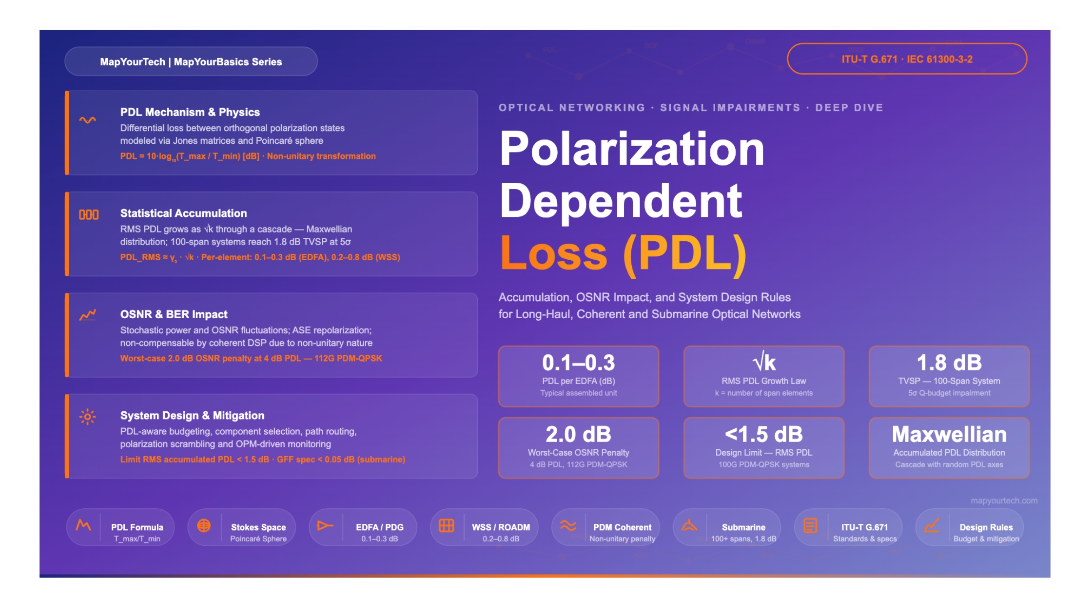
A comprehensive engineering reference covering the PDL mechanism, component-level values, statistical accumulation, OSNR and BER impacts, and practical system design guidelines for long-haul and coherent optical networks.

0.1–0.3 dB Typical per-component PDL (WDM filters, VOAs, OAs)
√k RMS PDL growth law — scales with number of spans k
1.8 dB Typical TVSP impairment in 100-span submarine system
2.0 dB Worst-case OSNR penalty at 4 dB PDL — 112G PDM-QPSK
Non-unitary PDL cannot be fully compensated by DSP — unlike PMD or CD
Maxwellian Statistical distribution of accumulated PDL in a cascade

1. Introduction

Light propagating through a single-mode optical fiber does so across two orthogonal polarization modes. In an ideal waveguide these two modes experience identical loss. In practice, every real optical component introduces some degree of differential loss between polarization states — a quantity known as Polarization Dependent Loss (PDL). While individually small, PDL contributions from many concatenated components accumulate across a long-haul or submarine link, producing stochastic power fluctuations and OSNR variations that can meaningfully degrade system performance.

PDL emerged as a design concern in parallel with the expansion of Dense Wavelength Division Multiplexing (DWDM) networks. As systems grew from a handful of amplifier spans to hundreds of spans in transoceanic cables, the statistical accumulation of small per-element PDL values became a budget item that system architects could not ignore. The problem intensified further with the shift to Polarization Division Multiplexed (PDM) coherent formats — 100G and beyond — because PDL induces orthogonality loss between the two polarization tributaries of a PDM signal, generating penalties that the digital signal processor (DSP) cannot fully recover.

This article provides a complete engineering treatment of PDL: its physical origin and mathematical formulation, typical values across component families, the statistical laws governing accumulation through a cascade, its impact on OSNR and bit error rate (BER), and practical design rules for managing PDL within a system margin budget. The analysis draws on ITU-T standards, established research, and real-world system data from submarine and terrestrial deployments.

Scope Clarification

This article addresses PDL in single-mode fiber systems employing conventional single-polarization and polarization-division-multiplexed (PDM) coherent formats. Polarization-Dependent Gain (PDG) in EDFAs, which has an equivalent effect to PDL, is also addressed where relevant. Polarization-Mode Dispersion (PMD), while related, is treated as a distinct impairment and discussed only in the context of its interaction with PDL.

2. Fundamental Principles of PDL

2.1 Physical Mechanism

PDL originates from the geometry and material properties of optical elements that interact differently with light depending on the orientation of its electric field vector — the state of polarization (SOP). The fundamental electromagnetic reason is that reflection, scattering, absorption, or coupling efficiency at an interface or within a waveguide depends on how the electric field aligns with the material's anisotropy axes.

In practice, PDL occurs in optical components such as isolators, optical couplers, WDM filters, wavelength-selective switches (WSSs), variable optical attenuators (VOAs), and optical amplifier passive components when the insertion loss varies with the SOPs of input signals. The effect is not limited to obviously polarization-sensitive components: even nominally symmetric components like fiber connectors and splices introduce small PDL values due to geometric imperfections, residual stress, or angular misalignment between fiber cores.

Critically, PDL is a passive, non-unitary transformation. Unlike PMD, which rotates the SOP without changing the total power, PDL changes the amplitude ratio between orthogonal polarization states. This non-unitary nature is precisely why PDL penalties cannot be undone by linear equalizers in a coherent DSP — some information content is irreversibly lost in the weaker polarization axis.

2.2 Mathematical Description

The most widely used definition of PDL quantifies it as the ratio between the maximum and minimum transmitted power for all possible input states of polarization. Expressed in decibels, PDL is:

/* PDL Definition — IEC 61300-3-2, ITU-T G.671 */

PDL = 10 · log10(Tmax / Tmin)   [dB]

Where:
  Tmax  =  Maximum transmittance over all input SOPs
  Tmin  =  Minimum transmittance over all input SOPs

Equivalent form using the PDL vector magnitude α:

PDL (Γ) = 10 · log10( (1 + α) / (1 - α) )   [dB]

Where:
  α = |α⃗|   (magnitude of the PDL vector in Stokes space)
  α⃗    =   PDL vector pointing toward the high-gain polarization state

/* Note: PDL ≥ 0 dB always; PDL = 0 means polarization-independent loss */

In the linear (non-dB) domain, the polarization-dependent component of the power gain of an optical component is described as 1 + α⃗ · ŝ, where ŝ is a unit Stokes vector corresponding to the SOP of the incident signal and α⃗ is the PDL vector. The highest and lowest gains are 1 ± α, achieved when the SOP is parallel or antiparallel to α⃗ in Stokes space.

2.3 PDL in Stokes and Jones Space

Two mathematical frameworks are used to analyze polarization effects in fiber systems: the Jones calculus and the Stokes/Mueller calculus.

In Jones space, a PDL element is represented by a non-unitary 2×2 Jones matrix. For a PDL element with attenuation axes aligned with the coordinate frame, the matrix takes the form:

/* Jones Matrix for PDL Element */

MPDL = [ 1      0  ]
         [ 0   e-Γ/2 ]

Where:
  Γ  =  PDL value in Nepers (natural units)
       (convert from dB: Γ_Np = PDL_dB × ln(10)/20)

/* For a cascade of N elements with random PDL axis orientations: */

Mtotal = MN · RN · MN-1 · RN-1 · ... · M1

Where:
  Ri  =  Unitary rotation matrix (random fiber birefringence between elements)
  Mi  =  Jones matrix of the i-th PDL element

The Stokes representation is particularly valuable for understanding PDL accumulation statistics because the overall PDL of a concatenated system, expressed in dB, follows a Maxwellian distribution when the individual elements have randomly oriented PDL axes — analogous to the Maxwellian distribution of PMD in long fibers.

Figure 1: PDL Physical Mechanism — Component Signal Flow and Poincaré Sphere Representation INPUT SIGNAL Arbitrary SOP Power: P₀ PDL ELEMENT (Isolator, Coupler, Filter, Connector) PDL = Γ dB HIGH GAIN AXIS T_max = (1+α)·P₀ SOP aligned to high-gain axis LOW GAIN AXIS T_min = (1−α)·P₀ SOP antiparallel to PDL vector PDL FORMULA PDL = 10·log₁₀(T_max / T_min) [dB] = 10·log₁₀( (1+α) / (1−α) ) α = PDL vector magnitude in Stokes space Cascade of PDL elements (distributed model): TX SOP₀ PDL₁ + R₁ PDL₂ + R₂ PDL_N + R_N RX OSNR↓ R_i = random polarization rotation (fiber birefringence between elements) Accumulated PDL (RMS) scales as √k where k = number of span elements S₃ (circular) S₂ S₁ Poincaré Sphere α (PDL vector) High-gain SOP Low-gain SOP SOP varies with time PDL Vector Properties High-gain SOP: parallel to α vector Low-gain SOP: antiparallel to α vector SOP drifts with time → stochastic power fluctuation at receiver Non-Unitary Nature PMD: unitary → DSP can compensate CD: deterministic → DSP can equalize PDL: non-unitary → NOT fully compensable Irreversible amplitude loss in one pol. axis
Figure 1: Left — Signal flow through a PDL element and cascade model. Right — Poincaré sphere representation showing the PDL vector, high-gain and low-gain SOPs, and the non-compensable nature of PDL.

3. PDL in Optical Components

Every optical component in a transmission line contributes a finite PDL value. Understanding the magnitude and source of PDL across different component families is the starting point for any system design exercise.

3.1 Passive Components

Optical connectors and splices are the most numerous PDL contributors in a system. PDL in connectors arises from fiber end-face geometry, angular misalignment between mating ferrules, and slight ellipticity of the fiber core at the interface. Well-polished UPC (Ultra Physical Contact) and APC (Angled Physical Contact) connectors typically contribute PDL in the range of 0.01–0.05 dB per mating pair, though values up to 0.1 dB are possible in field conditions. Fusion splices are generally lower, often below 0.01 dB when made with low-PMD fiber and competent field equipment.

Optical isolators use Faraday rotators and polarizers and are among the more significant sources of PDL. Their fundamental operating principle involves polarization-selective transmission, so even well-designed isolators carry PDL values in the range of 0.1–0.5 dB. Isolators are commonly found at the output of lasers, between amplifier stages, and before receivers.

WDM multiplexers and demultiplexers — whether thin-film filter (TFF) or arrayed waveguide grating (AWG) based — contribute PDL in the range of 0.1–0.5 dB per element. AWG devices tend to have lower PDL than TFF-based designs, but both are sensitive to manufacturing tolerances. In a DWDM add-drop network with several cascaded mux/demux elements, the accumulated PDL from this component family alone can reach 1–2 dB without careful selection.

Premium Article — Free 21% Preview

Read the Full Analysis with Premium

The remaining 79% of this article — the design numbers, trade-offs and field guidance — is part of MapYourTech Premium, along with the full premium library, courses and professional tools.


Instant access · Cancel anytime · 48-hour trial available
Sanjay Yadav

Optical Communications & Network Automation Expert | Author of 3 Books for Optical Engineers | Founder, MapYourTech

Optical networking engineer with nearly two decades of experience across DWDM, OTN, coherent optics, submarine systems, and cloud infrastructure. Founder of MapYourTech.

Follow on LinkedIn

You May Also Like

15 min read 14 0 Like Connector Types and Their Loss Budgets: SC, LC, MPO Skip to main content MapYourTech...
  • Free
  • July 11, 2026
16 min read 12 0 Like Cooled vs Uncooled Lasers: The Pluggable Power Trade-off Skip to main content MapYourTech |...
  • Free
  • July 11, 2026
16 min read 17 0 Like Automation Blast Radius: Scoping What a Bad Intent Can Touch Skip to main content...
  • Free
  • July 11, 2026

Course Title

Course description and key highlights

Course Content

Course Details
