
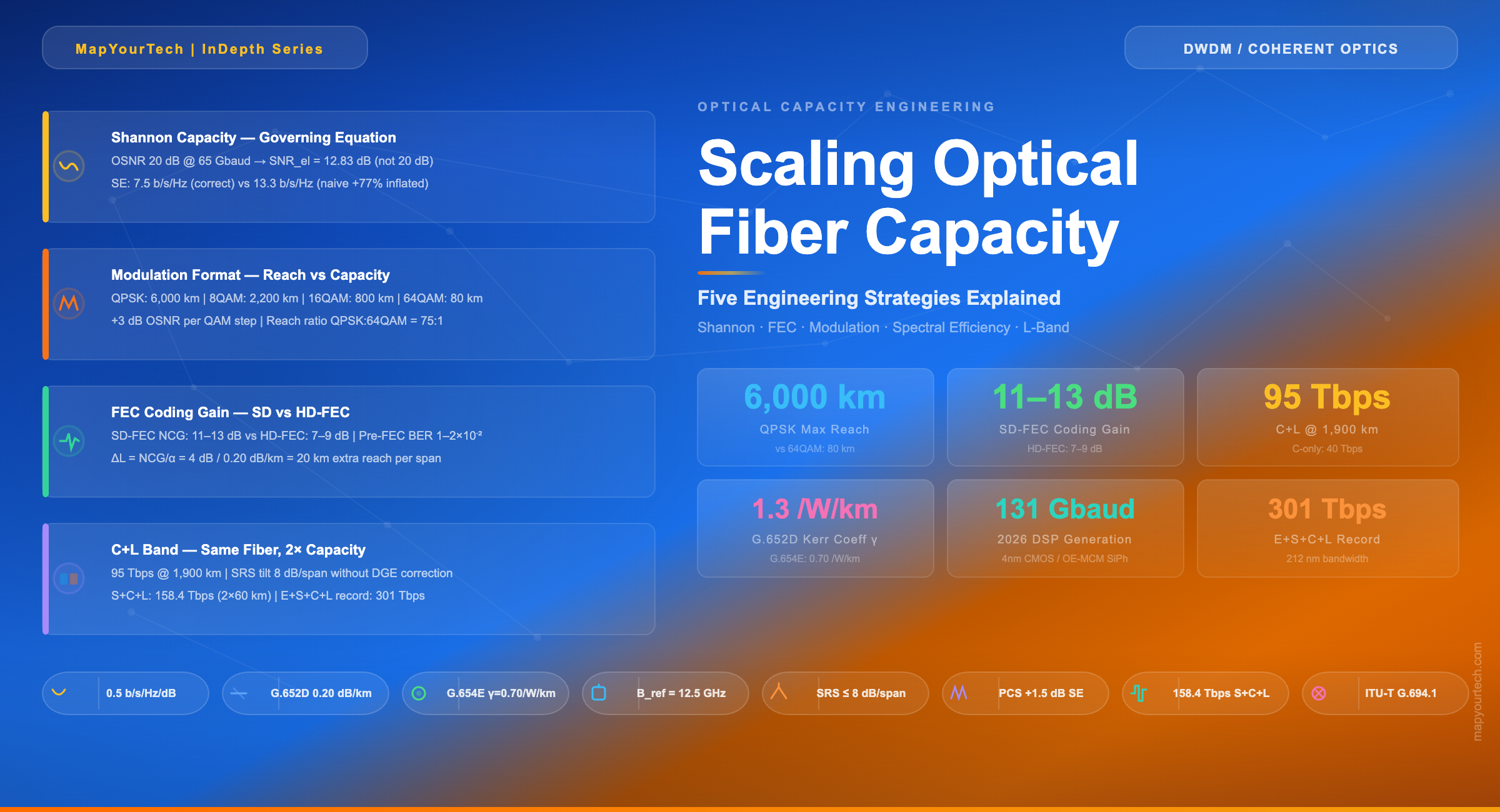
Optical Capacity Engineering Series — Comprehensive Deep Dive
Scaling Optical Fiber Capacity:
Five Engineering Strategies Explained
A complete technical guide covering how each capacity lever works, what it costs, and when to use it — Shannon capacity fundamentals, FEC coding gain, modulation trade-offs, spectral efficiency optimization, and C+L band expansion, with five interactive design tools and worked numerical examples throughout.
Table of Contents
1. Introduction
"The fiber is already in the ground. The question is how much of its capacity you are able to use — and at what cost."
— Andrew Chraplyvy, Bell Labs, pioneer of wavelength-division multiplexing
Every optical fiber is a physical channel bounded by immutable laws. The silica glass it is made from has a finite nonlinear refractive index. The erbium-doped amplifiers that sustain the signal over thousands of kilometers introduce noise with every gain stage. The dispersion coefficient of the fiber smears pulses across time. These are not engineering imperfections waiting to be designed away — they are properties of the material world that every optical network engineer must understand, quantify, and work within.
As of 2026, global IP traffic is growing at approximately 30–35% per year, compounding through hyperscale data center interconnection, 5G backhaul, submarine cable expansion, and AI inference workloads driving unprecedented traffic concentration in large-scale cloud infrastructure. The transition from 400G to 800G coherent pluggables is well underway: hyperscalers are deploying 800ZR/ZR+ modules in large volumes, and service providers are accelerating IP-over-DWDM upgrades using 400G pluggables. This traffic growth consistently outpaces the economics of deploying new fiber — especially on submarine routes where a single transoceanic cable system can cost $300M or more to build. The only sustainable response is to extract more capacity from fiber that is already in the ground, using the five physics-constrained architectural strategies this article analyzes in depth.
The five strategies are: widening the per-channel bandwidth through higher baud rates, improving forward error correction (FEC) coding gain, using higher-order modulation formats to pack more bits per symbol, optimizing spectral efficiency through better fiber design and digital nonlinear compensation, and expanding into the L-band to access new optical spectrum. Each strategy has a direct physical basis, a quantifiable return, and a price that must be paid. Understanding the correlations between them — how they interact through the shared parameters of OSNR budget, nonlinear tolerance, and amplification bandwidth — is the foundation of every sound long-haul and submarine system design.
Capacity Architecture Map
Five Engineering Levers — How They Interact
All five levers interact through the shared OSNR budget. Bandwidth expansion (①④) scales linearly. SNR-based levers (②③⑤) obey the 0.5 b/s/Hz/dB Shannon slope.
This article is structured for the practicing engineer: each section opens with a real industry or research quote establishing context, develops the mechanism from first principles with verified numerical data, presents both advantages and challenges honestly, and connects the strategy to the others through explicit correlations. Five embedded interactive tools allow you to calculate Shannon capacity, OSNR link budgets, modulation trade-offs, FEC gain impacts, and C+L band capacity directly within the article.
2. The Shannon Foundation — The Governing Equation
"The fundamental problem of communication is that of reproducing at one point either exactly or approximately a message selected at another point."
— Claude E. Shannon, A Mathematical Theory of Communication, Bell System Technical Journal
Shannon's theorem establishes the maximum rate at which information can be transmitted reliably over a noisy channel of given bandwidth and signal-to-noise ratio. For a polarization-multiplexed single-mode fiber channel — the standard configuration for all coherent DWDM systems — the theoretical capacity limit is:
C = 2 × Rₛ × log₂(1 + SNRₛₛ)

Where:
  C      = theoretical maximum channel capacity (bits/s)
  Rₛ     = baud rate  [= Slot_width / (1 + roll-off)]  — NOT the slot width
  SNRₛₛ  = electrical Eₛ/N₀ per polarization  — NOT optical OSNR
  2      = PDM factor: two orthogonal polarization modes

⚠ IMPORTANT — Two corrections vs naive application:
  1. B in Shannon = baud rate Rₛ, NOT slot width
     Rₛ = Slot_width / (1 + roll-off)
  2. SNR in Shannon = per-pol electrical Eₛ/N₀, NOT optical OSNR
     SNRₛₛ = OSNR_lin × (B_ref / Rₛ)  where B_ref = 12.5 GHz (0.1 nm ref BW)

Worked Example — 75 GHz flex-grid channel, OSNR = 20 dB (0.1 nm), roll-off = 0.15:

  Step 1 — Baud rate from slot:
    Rₛ = 75 GHz / (1 + 0.15) = 65.2 Gbaud

  Step 2 — Convert OSNR to electrical Eₛ/N₀:
    OSNR_lin = 10^(20/10) = 100.0 (linear)
    SNRₛₛ = 100.0 × (12.5 / 65.2) = 19.17 linear → 12.83 dB
    Note: the OSNR→Eₛ/N₀ penalty = 10×log₁₀(12.5/65.2) = −7.17 dB

  Step 3 — Apply Shannon:
    C = 2 × 65.2 × log₂(1 + 19.17)
      = 2 × 65.2 × log₂(20.17)
      = 2 × 65.2 × 4.335 = 565 Gbps

  Step 4 — Spectral efficiency:
    SE_slot = 565 / 75 GHz = 7.53 b/s/Hz  (relative to channel slot)
    SE_baud = 565 / 65.2 GHz = 8.67 b/s/Hz  (relative to baud rate)

  What would WRONG naive calculation give?
    C_naive = 2 × 75 GHz × log₂(1 + 100) = 2 × 75 × 6.66 = 999 Gbps
    SE_naive = 999/75 = 13.3 b/s/Hz
    Error factor: 999/565 = 1.77× too optimistic (77% inflated)

  Deployed 400G DP-16QAM in 75 GHz: SE_dep = 400/75 = 5.33 b/s/Hz
  Shannon ceiling (correct): 7.53 b/s/Hz
  Gap to Shannon: 7.53 - 5.33 = 2.20 b/s/Hz (being closed by PCS + SD-FEC)
Interactive Tool 1 of 5
Shannon Capacity Explorer — Corrected Full-Factor Model
Uses the full optical Shannon model: slot width → baud rate via roll-off, OSNR → electrical Es/N₀ conversion (Bref = 12.5 GHz), implementation margin, and PDM factor. The chart shows Shannon SE (b/s/Hz) vs OSNR with modulation format reference lines at their practical achieved SE values.
Spectral Parameters
SNR / Noise Parameters
System Parameters
Derived Values
Shannon SE (b/s/Hz) vs OSNR — with modulation format reference lines
3. The Five Physics-Forcing Strategies — In Depth
The five strategies address different physical dimensions of the capacity equation. Wider channels and L-band expansion attack the bandwidth term B directly. Better FEC and higher modulation address the log₂(1 + SNR) term — FEC by improving the effective SNR margin available to the system, modulation by packing more information per unit of SNR. Spectral efficiency optimization — through better fiber, DSP nonlinear compensation, and Raman amplification — improves both dimensions simultaneously by reducing the noise and impairment floor. Each is examined in detail below.
Read the Full Analysis with Premium
The remaining 89% of this article — the design numbers, trade-offs and field guidance — is part of MapYourTech Premium, along with the full premium library, courses and professional tools.
You May Also Like

-
Free
-
September 4, 2026

-
Premium
-
September 4, 2026

-
Premium
-
September 4, 2026